10.3 Variable selection property of the lasso
You may ask why lasso (\(L_1\) penalty) has the feature selection property but not the ridge (\(L_2\) penalty). To answer that question, let’s look at the alternative representations of the optimization problem for lasso and ridge. For lasso regression, it is identical to optimize the following two functions:
\[\begin{equation} \Sigma_{i=1}^{n}(y_{i}-\beta_{0}-\Sigma_{j=1}^{p}\beta_{j}x_{ij})^{2}+\lambda\Sigma_{j=1}^{p}|\beta_{j}|=RSS+\lambda\Sigma_{j=1}^{p}|\beta_{j}| \tag{10.3} \end{equation}\]
\[\begin{equation} \underset{\beta}{min}\left\{ \Sigma_{i=1}^{n}\left(y_{i}-\beta_{0}-\Sigma_{j=1}^{p}\beta_{j}x_{ij}\right)^{2}\right\} ,\ \Sigma_{j=1}^{p}|\beta_{j}|\leq s \tag{10.4} \end{equation}\]
For any value of tuning parameter \(\lambda\), there exists a \(s\) such that the coefficient estimates optimize equation (10.3) also optimize equation (10.4). Similarly, for ridge regression, the two representations are identical:
\[\begin{equation} \Sigma_{i=1}^{n}(y_{i}-\beta_{0}-\Sigma_{j=1}^{p}\beta_{j}x_{ij})^{2}+\lambda\Sigma_{j=1}^{p}\beta_{j}^{2}=RSS+\lambda\Sigma_{j=1}^{p}\beta_{j}^{2} \tag{10.5} \end{equation}\]
\[\begin{equation} \underset{\beta}{min}\left\{ \Sigma_{i=1}^{n}\left(y_{i}-\beta_{0}-\Sigma_{j=1}^{p}\beta_{j}x_{ij}\right)^{2}\right\} ,\ \Sigma_{j=1}^{p}\beta_{j}^{2}\leq s \tag{10.6} \end{equation}\]
When \(p=2\), lasso estimates (\(\hat{\beta}_{lasso}\) in figure 10.3) have the smallest RSS among all points that satisfy \(|\beta*{1}|+|\beta_{2}|\leq s\) (i.e. within the diamond in figure 10.3). Ridge estimates have the smallest RSS among all points that satisfy \(\beta_{1}^{2}+\beta_{2}^{2}\leq s\) (i.e. within the circle in figure 10.3). As s increases, the diamond and circle regions expand and get less restrictive. If s is large enough, the restrictive region will cover the least squares estimate (\(\hat{\beta}_{LSE}\)). Then, equations (10.4) and (10.6) will simply yield the least squares estimate. In contrast, if s is small, the grey region in figure 10.3 will be small and hence restrict the magnitude of \(\beta\). With the alternative formulations, we can answer the question of feature selection property.
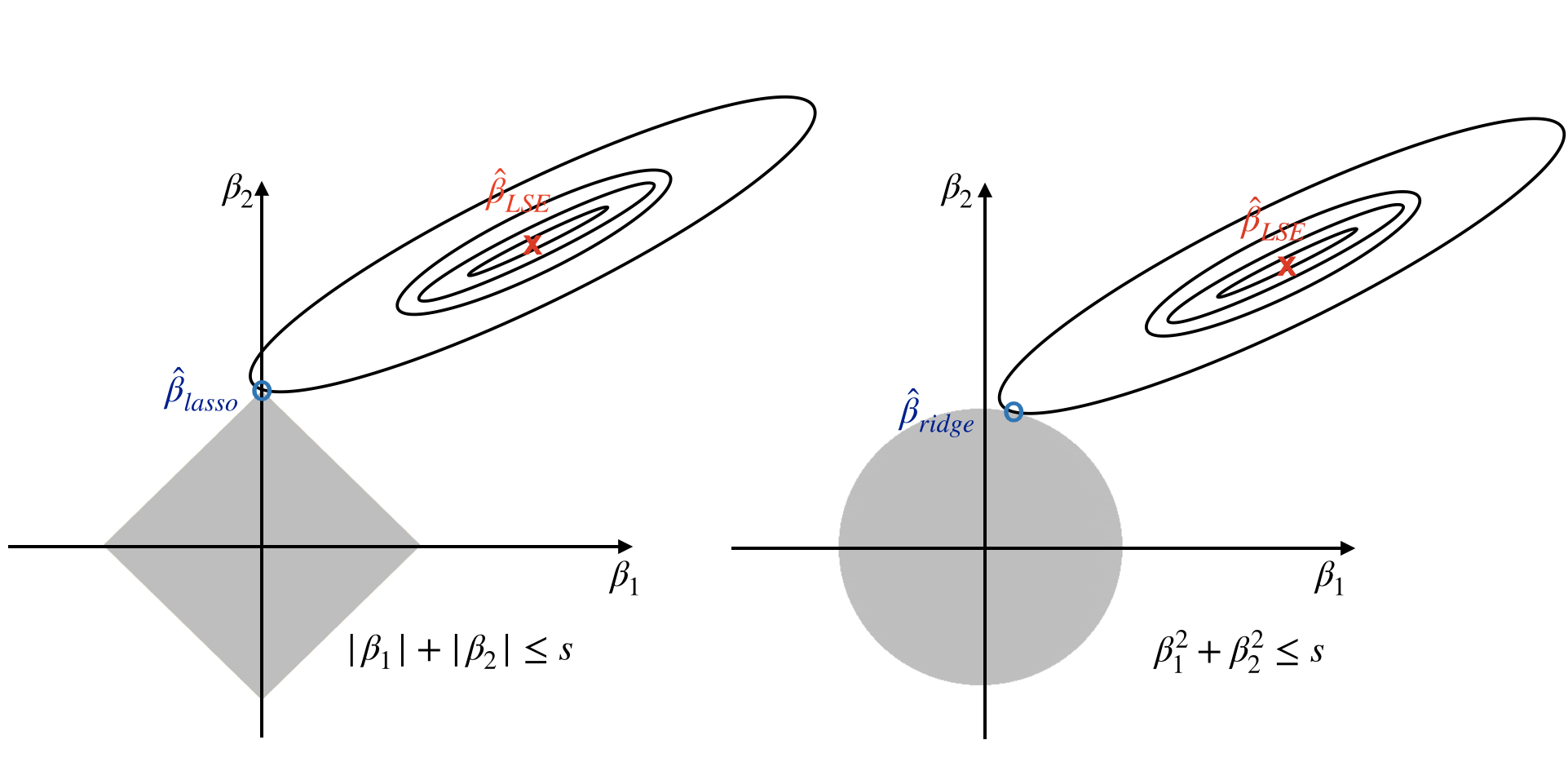
FIGURE 10.3: Contours of the RSS and constrain functions for the lasso (left) and ridge regression (right)
Figure 10.3 illustrates the situations for lasso (left) and ridge (right). The least square estimate is marked as \(\hat{\beta}\). The restrictive regions are in grey, the diamond region is for the lasso, the circle region is for the ridge. The least square estimates lie outside the grey region, so they are different from the lasso and ridge estimates. The ellipses centered around \(\hat{\beta}\) represent contours of RSS. All the points on a given ellipse share an RSS. As the ellipses expand, the RSS increases. The lasso and ridge estimates are the first points at which an ellipse contracts the grey region. Since ridge regression has a circular restrictive region that doesn’t have a sharp point, the intersecting point can’t drop on the axis. But it is possible for lasso since it has corners at each of the axes. When the intersecting point is on an axis, one of the parameter estimates is 0. If p > 2, the restrictive regions become sphere or hypersphere. In that case, when the intersecting point drops on an axis, multiple coefficient estimates can equal 0 simultaneously.