11.1 Tree Basics
The tree-based models can be used for regression and classification. The goal is to stratify or segment the predictor space into a number of sub-regions. For a given observation, use the mean (regression) or the mode (classification) of the training observations in the sub-region as the prediction. Tree-based methods are conceptually simple yet powerful. This type of model is often referred to as Classification And Regression Trees (CART). They are popular tools for many reasons:
- Do not require user to specify the form of the relationship between predictors and response
- Do not require (or if they do, very limited) data preprocessing and can handle different types of predictors (sparse, skewed, continuous, categorical, etc.)
- Robust to co-linearity
- Can handle missing data
- Many pre-built packages make implementation as easy as a button push
CART can refer to the tree model in general, but most of the time, it represents the algorithm initially proposed by Breiman (L. Breiman et al. 1984). After Breiman, there are many new algorithms, such as ID3, C4.5, and C5.0. C5.0 is an improved version of C4.5, but since C5.0 is not open source, the C4.5 algorithm is more popular. C4.5 was a major competitor of CART. But now, all those seem outdated. The most popular tree models are Random Forest (RF) and Gradient Boosting Machine (GBM). Despite being out of favor in application, it is important to understand the mechanism of the basic tree algorithm. Because the later models are based on the same foundation.
The original CART algorithm targets binary classification, and the later algorithms can handle multi-category classification. A single tree is easy to explain but has poor accuracy. More complicated tree models, such as RF and GBM, can provide much better prediction at the cost of explainability. As the model becoming more complicated, it is more like a black-box which makes it very difficult to explain the relationship among predictors. There is always a trade-off between explainability and predictability.
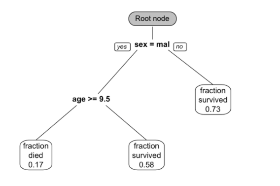
FIGURE 11.1: This is a classification tree trained from passenger survival data from the Titanic. Survival probability is predicted using sex and age.
The reason why it is called “tree” is of course because the structure has similarities. But the direction of the decision tree is opposite of a real tree, the root is on the top, and the leaf is on the bottom (figure 11.1). From the root node, a decision tree divides to different branches and generates more nodes. The new nodes are child nodes, and the previous node is the parent node. At each child node, the algorithm will decide whether to continue dividing. If it stops, the node is called a leaf node. If it continues, then the node becomes the new parent node and splits to produce the next layer of child nodes. At each non-leaf node, the algorithm needs to decide if it will split into branches. A leaf node contains the final “decision” on the sample’s value. Here are the important definitions in the tree model:
- Classification tree: the outcome is discrete
- Regression tree: the outcome is continuous (e.g. the price of a house)
- Non-leaf node (or split node): the algorithm needs to decide a split at each non-leaf node (eg: age >= 9.5)
- Root node: the beginning node where the tree starts
- Leaf node (or Terminal node): the node stops splitting. It has the final decision of the model
- Degree of the node: the number of subtrees of a node
- Degree of the tree: the maximum degree of a node in the tree
- Pruning: remove parts of the tree that do not provide power to classify instances
- Branch (or Subtree): the whole part under a non-leaf node
- Child node: the node directly after and connected to another node
- Parent node: the converse notion of a child
A single tree is easy to explain, but it can be very non-robust, which means a slight change in the data can significantly change the fitted tree. The predictive accuracy is not as good as other regression and classification approaches in this book since a series of rectangular decision regions defined by a single tree is often too naive to represent the relationship between the dependent variable and the predictors. Figure 11.2 shows an example of decision regions based on the iris data in R where we use petal length (Petal.Length) and width (Petal.Width) to decide the type of flowers (Species). You can get the data frame using the following code:
data("iris")
head(iris)
## Sepal.Length Sepal.Width Petal.Length Petal.Width
## 1 5.1 3.5 1.4 0.2
## 2 4.9 3.0 1.4 0.2
## 3 4.7 3.2 1.3 0.2
## 4 4.6 3.1 1.5 0.2
## 5 5.0 3.6 1.4 0.2
## 6 5.4 3.9 1.7 0.4
## Species
## 1 setosa
## 2 setosa
## 3 setosa
## 4 setosa
## 5 setosa
## 6 setosaTo overcome these shortcomings, researchers have proposed ensemble methods which combine many trees. Ensemble tree models typically have much better predictive performance than a single tree. We will introduce those models in later sections.
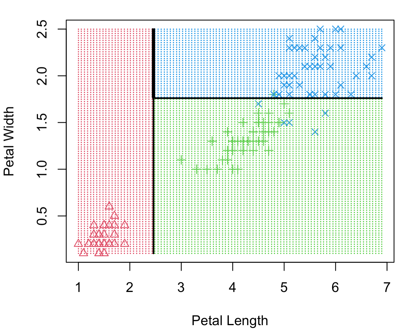
FIGURE 11.2: Example of decision regions for different types of flowers based on petal length and width. Three different types of flowers are classified using decisions about length and width.