11.2 Splitting Criteria
The splitting criteria used by the regression tree and the classification tree are different. Like the regression tree, the goal of the classification tree is to divide the data into smaller, more homogeneous groups. Homogeneity means that most of the samples at each node are from one class. The original CART algorithm uses Gini impurity as the splitting criterion; The later ID3, C4.5, and C5.0 use entropy. We will look at three most common splitting criteria.
11.2.1 Gini impurity
Gini impurity (L. Breiman et al. 1984) is a measure of non-homogeneity. It is widely used in classification tree. It is defined as: \[Gini\ Index = \Sigma_i p_i(1-p_i)\]
where \(p_i\) is the probability of class \(i\) and the interval of Gini is \([0, 0.5]\). For a two-class problem, the Gini impurity for a given node is:
\[p_{1}(1-p_{1})+p_{2}(1-p_{2})\]
It is easy to see that when the sample set is pure, one of the probability is 0 and the Gini score is the smallest. Conversely, when \(p_{1} = p_{2} = 0.5\), the Gini score is the largest, in which case the purity of the node is the smallest. Let’s look at an example. Suppose we want to determine which students are computer science (CS) majors. Here is the simple hypothetical classification tree result obtained with the gender variable.
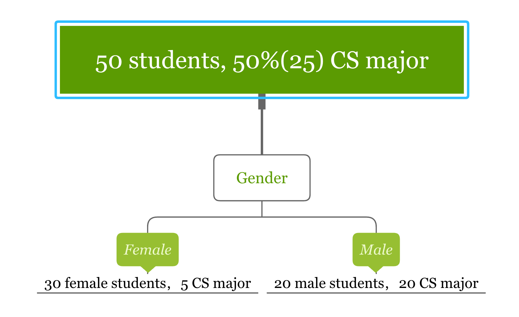
Let’s calculate the Gini impurity for splitting node “Gender”:
- Gini impurity for “Female” = \(\frac{1}{6}\times\frac{5}{6}+\frac{5}{6}\times\frac{1}{6}=\frac{5}{18}\)
- Gini impurity for “Male” = \(0\times1+1\times 0=0\)
The Gini impurity for the node “Gender” is the following weighted average of the above two scores:
\[\frac{3}{5}\times\frac{5}{18}+\frac{2}{5}\times 0=\frac{1}{6}\]
The Gini impurity for the 50 samples in the parent node is \(\frac{1}{2}\). It is easy to calculate the Gini impurity drop from \(\frac{1}{2}\) to \(\frac{1}{6}\) after splitting. The split using “gender” causes a Gini impurity decrease of \(\frac{1}{3}\). The algorithm will use different variables to split the data and choose the one that causes the most substantial Gini impurity decrease.
11.2.2 Information Gain (IG)
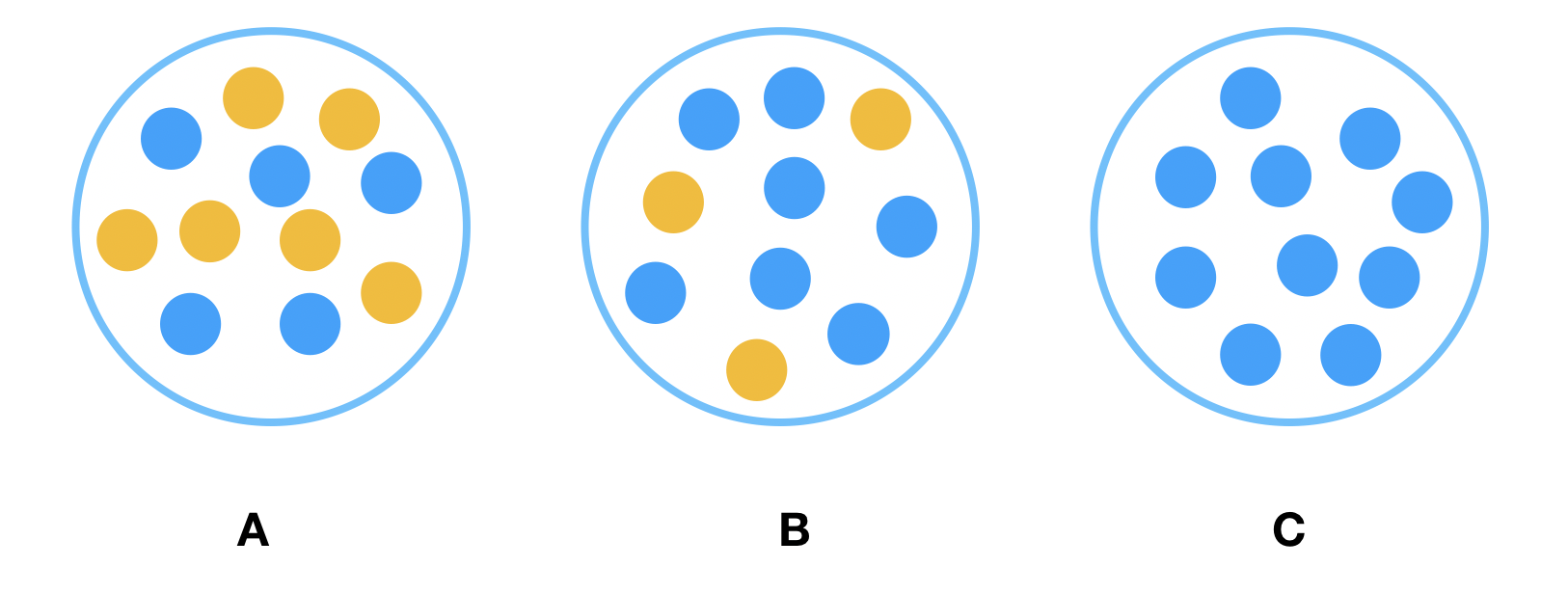
Looking at the samples in the following three nodes, which one is the easiest to describe? It is obviously C. Because all the samples in C are of the same type, so the description requires the least amount of information. On the contrary, B needs more information, and A needs the most information. In other words, C has the highest purity, B is the second, and A has the lowest purity. We need less information to describe nodes with higher purity.
A measure of the degree of disorder is entropy which is defined as:
\[Entropy = - \Sigma_i p_i log_2(p_i)\] where \(p_i\) is the probability of class \(i\) and the interval of entropy is \([0, 1]\). For a two-class problem:
\[Entropy=-plog_{2}p-(1-p)log_{2}(1-p)\]
where p is the percentage of one type of samples. If all the samples in one node are of one type (such as C), the entropy is 0. If the proportion of each type in a node is 50%, the entropy is 1. We can use entropy as splitting criteria. The goal is to decrease entropy as the tree grows. As an analogy, entropy in physics quantifies the level of disorder and the goal here is to have the least disorder.
Similarly, the entropy of a splitting node is the weighted average of the entropy of each child. In the above tree for the students, the entropy of the root node with all 50 students is \(-\frac{25}{50}log_{2}\frac{25}{50}-\frac{25}{50}log_{2}\frac{25}{50}=1\). Here an entropy of 1 indicates that the purity of the node is the lowest, that is, each type takes up half of the samples.
The entropy of the split using variable “gender” can be calculated in three steps:
- Entropy for “Female” = \(-\frac{5}{30}log_{2}\frac{5}{30}-\frac{25}{30}log_{2}\frac{25}{30}=0.65\)
- Entropy for “Male” = \(0\times1+1\times 0=0\)
- Entropy for the node “Gender” is the weighted average of the above two entropy numbers: \(\frac{3}{5}\times 0.65+\frac{2}{5}\times 0=0.39\)
So entropy decreases from 1 to 0.39 after the split and the IG for “Gender” is 0.61.
11.2.3 Information Gain Ratio (IGR)
ID3 uses information gain as the splitting criterion to train the classification tree. A drawback of information gain is that it is biased towards choosing attributes with many values, resulting in overfitting (selecting a feature that is non-optimal for prediction) (HSSINA et al. 2014).
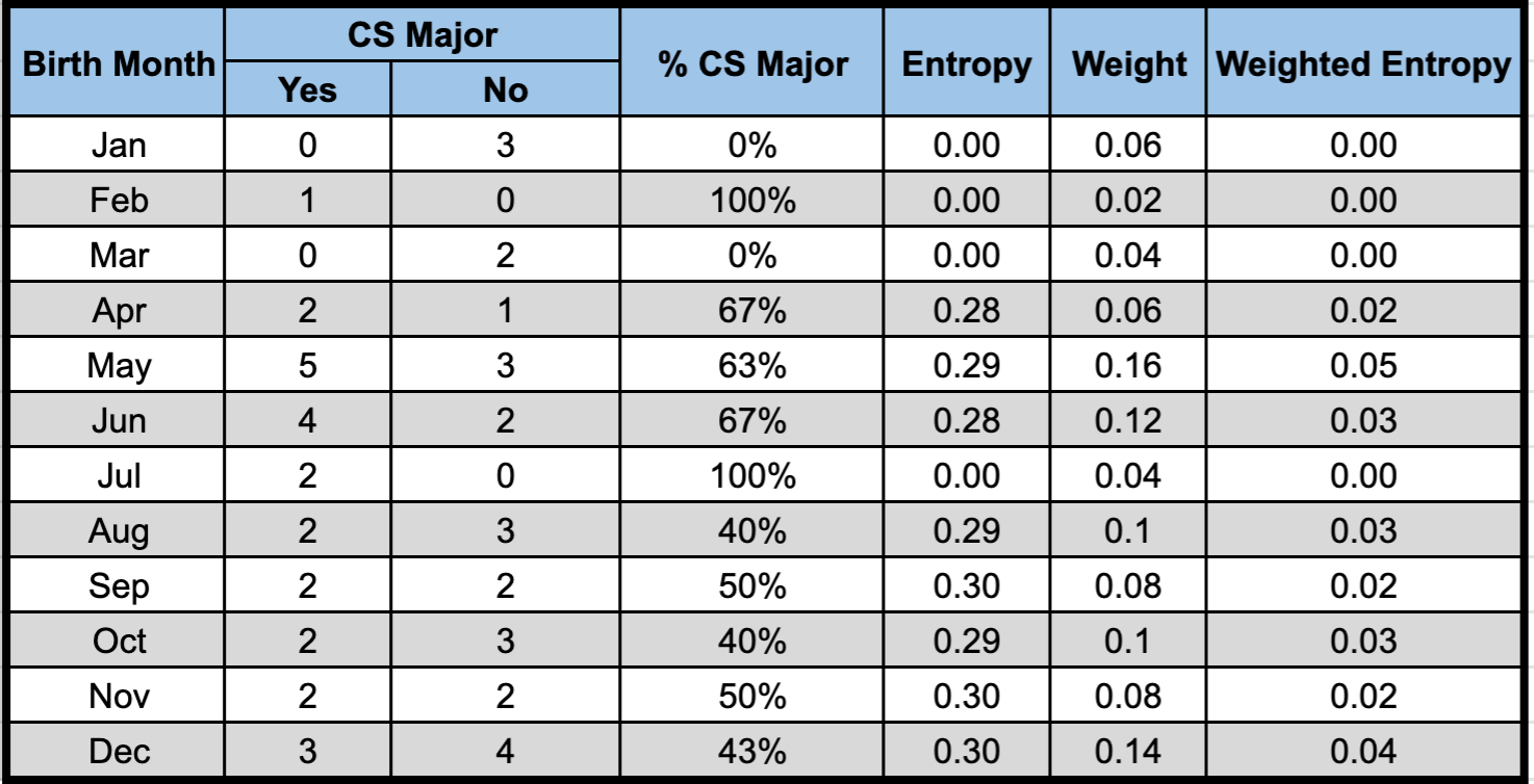
To understand why let’s look at another hypothetical scenario. Assume that the training set has students’ birth month as a feature. You might say that the birth month should not be considered in this case because it intuitively doesn’t help tell the student’s major. Yes, you’re right. However, practically, we may have a much more complicated dataset, and we may not have such intuition for all the features. So, we may not always be able to determine whether a feature makes sense or not. If we use the birth month to split the data, the corresponding entropy of the node “Birth Month” is 0.24 (the sum of column “Weighted Entropy” in the table), and the information gain is 0.76, which is larger than the IG of “Gender” (0.61). So between the two features, IG would choose “Birth Month” to split the data.
To overcome this problem, C4.5 uses the “information gain ratio” instead of “information gain.” The gain ratio is defined as:
\[Gain\ Ratio = \frac{Information\ Gain}{Split\ Information}\] where split information is:
\[Split\ Information = -\Sigma_{c = 1}^{C}p_clog(p_c)\] \(p_c\) is the proportion of samples in category \(c\). For example, there are three students with the birth month in Jan, 6% of the total 50 students. So the \(p_c\) for “Birth Month = Jan” is 0.06. The split information measures the intrinsic information that is independent of the sample distribution inside different categories. The gain ratio corrects the IG by taking the intrinsic information of a split into account.
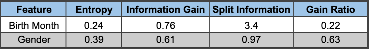
The split information for the birth month is 3.4, and the gain ratio is 0.22, which is smaller than that of gender (0.63). The gain ratio refers to use gender as the splitting feature rather than the birth month. Gain ratio favors attributes with fewer categories and leads to better generalization (less overfitting).
11.2.4 Sum of Squared Error (SSE)
The previous two metrics are for classification tree. The SSE is the most widely used splitting metric for regression. Suppose you want to divide the data set \(S\) into two groups of \(S_{1}\) and \(S_{2}\), where the selection of \(S_{1}\) and \(S_{2}\) needs to minimize the sum of squared errors:
\[\begin{equation} SSE=\Sigma_{i\in S_{1}}(y_{i}-\bar{y}_{1})^{2}+\Sigma_{i\in S_{2}}(y_{i}-\bar{y}_{2})^{2} \tag{11.1} \end{equation}\]
In equation (11.1), \(\bar{y}_{1}\) and \(\bar{y}_{2}\) are the average of the sample in \(S_{1}\) and \(S_{2}\). The way regression tree grows is to automatically decide on the splitting variables and split points that can maximize SSE reduction. Since this process is essentially a recursive segmentation, this approach is also called recursive partitioning.
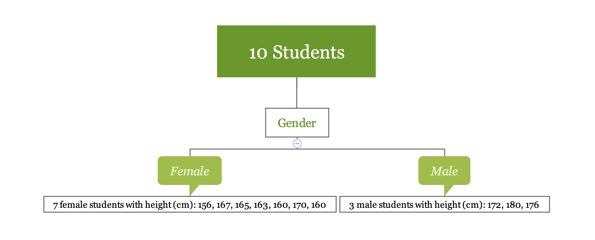
Take a look at this simple regression tree for the height of 10 students:
You can calculate the SSE using the following code:
- SSE for “Female” is 136
- SSE for “Male” is 32
- SSE for splitting node “Gender” is the sum of the above two numbers which is 168
SSE for the 10 students in root node is 522.9. After the split, SSE decreases from 522.9 to 168.
If there is another possible way of splitting, divide it by major, as follows:
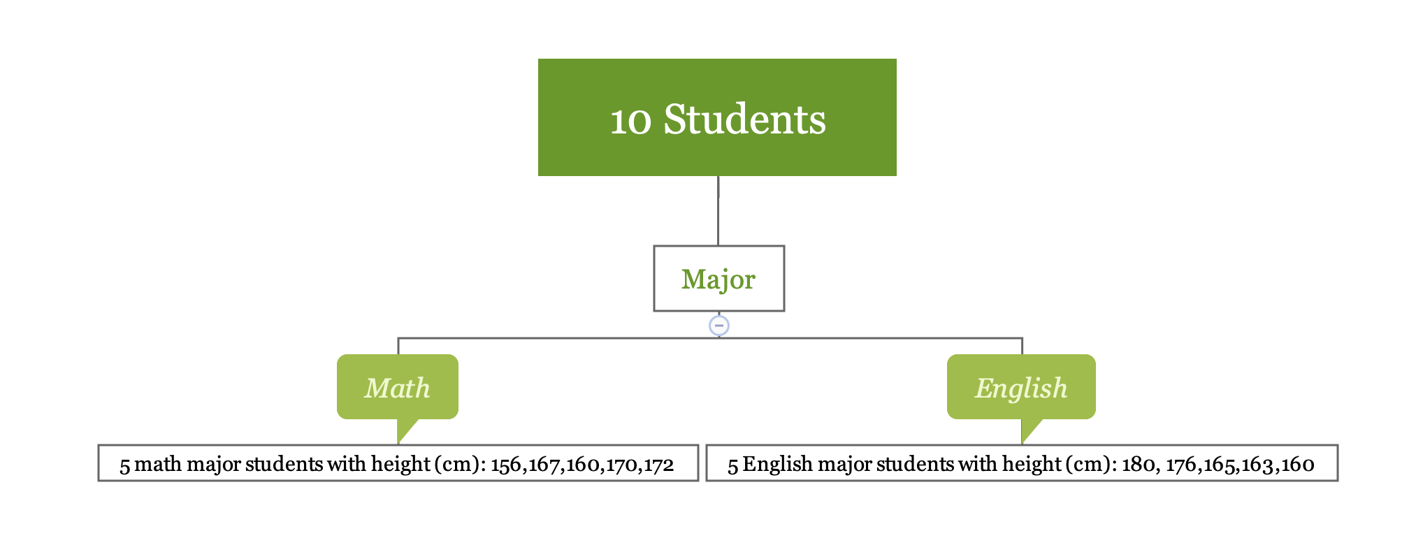
In this situation:
- SSE for “Math” is 184
- SSE for “English” is 302.8
- SSE for splitting node “Major” is the sum of the above two numbers which is 486.8
Splitting data using variable “gender” reduced SSE from 522.9 to 168; using variable “major” reduced SSE from 522.9 to 486.8. Based on SSE reduction, you should use gender to split the data.
The three splitting criteria mentioned above are the basis for building a tree model.