4.1 Power of Cluster of Computers
We are familiar with our laptop/desktop computers which have three main components to do data computation: (1) Hard disk, (2) Memory, and (3) CPU.
The data and codes stored in the hard disk have specific features such as slow to read and write, and large capacity of around a few TB in today’s market. Memory is fast to read and write but with small capacity in the order of a few dozens of GB in today’s market. CPU is where all the computation happens.
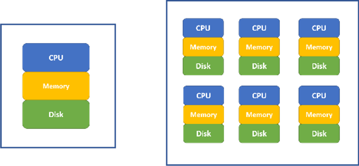
FIGURE 4.1: Single computer (left) and a cluster of computers (right)
For statistical software such as R, the amount of data it can process is limited by the computer’s memory. The memory of computers before 2000 is less than 1 GB. The memory capacity grows way slower than the amount of the data. Now it is common that we need to analyze data far beyond the capacity of a single computer’s memory, especially in an enterprise environment. Meanwhile, as the data size increases, to solve the same problem (such as regressions), the computation time is growing faster than linear. Using a cluster of computers become a common way to solve a big data problem. In figure 4.1 (right), a cluster of computers can be viewed as one powerful machine with memory, hard disk and CPU equivalent to the sum of individual computers. It is common to have hundreds or even thousands of nodes for a cluster.
In the past, users need to write code (such as MPI) to distribute data and do parallel computing. Fortunately, with the recent new development, the cloud environment for big data analysis is more user-friendly. As data is often beyond the size of the hard disk, the dataset itself is stored across different nodes (i.e., the Hadoop system). When doing analysis, the data is distributed across different nodes, and algorithms are parallel to leverage corresponding nodes’ CPUs to compute (i.e., the Spark system).