12.1 Feedforward Neural Network
12.1.1 Logistic Regression as Neural Network
Let’s look at logistic regression from the lens of the neural network. For a binary classification problem, for example spam classifier, given \(m\) samples \(\{(x^{(1)}, y^{(1)}),(x^{(2)}, y^{(2)}),...,(x^{(m)}, y^{(m)})\}\), we need to use the input feature \(x^{(i)}\) (they may be the frequency of various words such as “money”, special characters like dollar signs, and the use of capital letters in the message etc.) to predict the output \(y^{(i)}\) (if it is a spam email). Assume that for each sample \(i\), there are \(n_{x}\) input features. Then we have:
\[\begin{equation} X=\left[\begin{array}{cccc} x_{1}^{(1)} & x_{1}^{(2)} & \dotsb & x_{1}^{(m)}\\ x_{2}^{(1)} & x_{2}^{(2)} & \dotsb & x_{2}^{(m)}\\ \vdots & \vdots & \vdots & \vdots\\ x_{n_{x}}^{(1)} & x_{n_{x}}^{(2)} & \dots & x_{n_{x}}^{(m)} \end{array}\right]\in\mathbb{R}^{n_{x}\times m} \tag{12.1} \end{equation}\]
\[y=[y^{(1)},y^{(2)},\dots,y^{(m)}] \in \mathbb{R}^{1 \times m}\]
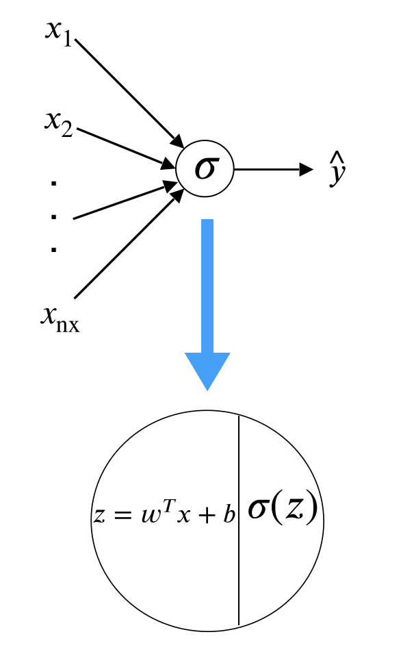
To predict if sample \(i\) is a spam email, we first get the inactivated neuro \(z^{(i)}\) by a linear transformation of the input \(x^{(i)}\), which is \(z^{(i)}=w^Tx^{(i)} + b\). Then we apply a function to “activate” the neuro \(z^{(i)}\) and we call it “activation function”. In logistic regression, the activation function is sigmoid function and the “activated” \(z^{(i)}\) is the prediction:
\[\hat{y}^{(i)} = \sigma(w^Tx^{(i)} + b)\]
where \(\sigma(z) = \frac{1}{1+e^{-z}}\). The following figure summarizes the process:
There are two types of layers. The last layer connects directly to the output. All the rest are intermediate layers. Depending on your definition, we call it “0-layer neural network” where the layer count only considers intermediate layers. To train the model, you need a cost function which is defined as equation (12.2).
\[\begin{equation} J(w,b)=\frac{1}{m} \Sigma_{i=1}^m L(\hat{y}^{(i)}, y^{(i)}) \tag{12.2} \end{equation}\]
where
\[L(\hat{y}^{(i)}, y^{(i)}) = -y^{(i)}log(\hat{y}^{(i)})-(1-y^{(i)})log(1-\hat{y}^{(i)})\]
To fit the model is to minimize the cost function.
12.1.2 Stochastic Gradient Descent
The general approach to minimize \(J(w,b)\) is by gradient descent, also known as back-propagation. The optimization process is a forward and backward sweep over the network.
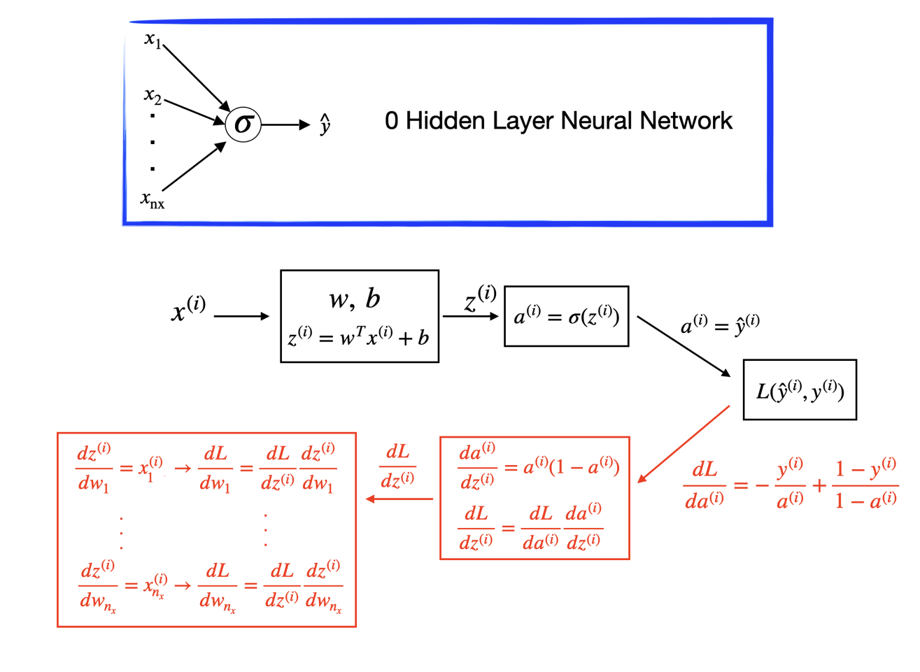
The forward propagation takes the current weights, calculates the prediction and cost. The backward propagation computes the gradient descent for the parameters by the chain rule for differentiation. In logistic regression, it is easy to calculate the gradient w.r.t the parameters \((w, b)\).
Let’s look at the Stochastic Gradient Descent (SGD) for logistic regression across \(m\) samples. SGD updates one sample each time. The detailed process is as follows.
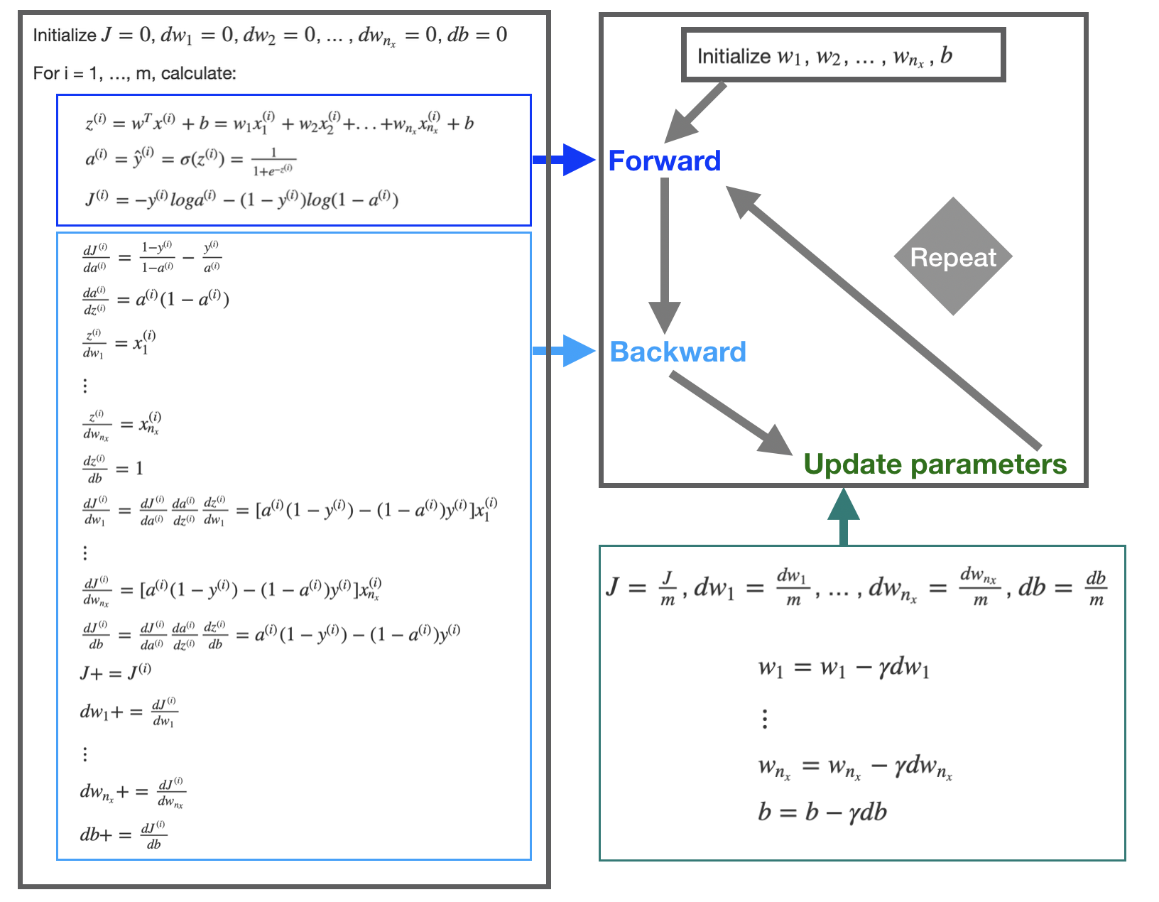
First initialize \(w_1\), \(w_2\), … , \(w_{n_x}\), and \(b\). Then plug in the initialized value to the forward and backward propagation. The forward propagation takes the current weights and calculates the prediction \(\hat{h}^{(i)}\) and cost \(J^{(i)}\). The backward propagation calculates the gradient descent for the parameters. After iterating through all \(m\) samples, you can calculate gradient descent for the parameters. Then update the parameter by: \[w := w - \gamma \frac{\partial J}{\partial w}\] \[b := b - \gamma \frac{\partial J}{\partial b}\]
Repeat the forward and backward process using the updated parameter until the cost \(J\) stabilizes.
12.1.3 Deep Neural Network
Before people coined the term deep learning, a neural network refers to single hidden layer network. Neural networks with more than one layers are called deep learning. Network with the structure in figure 12.1 is the multiple layer perceptron (MLP) or feedforward neural network (FFNN).
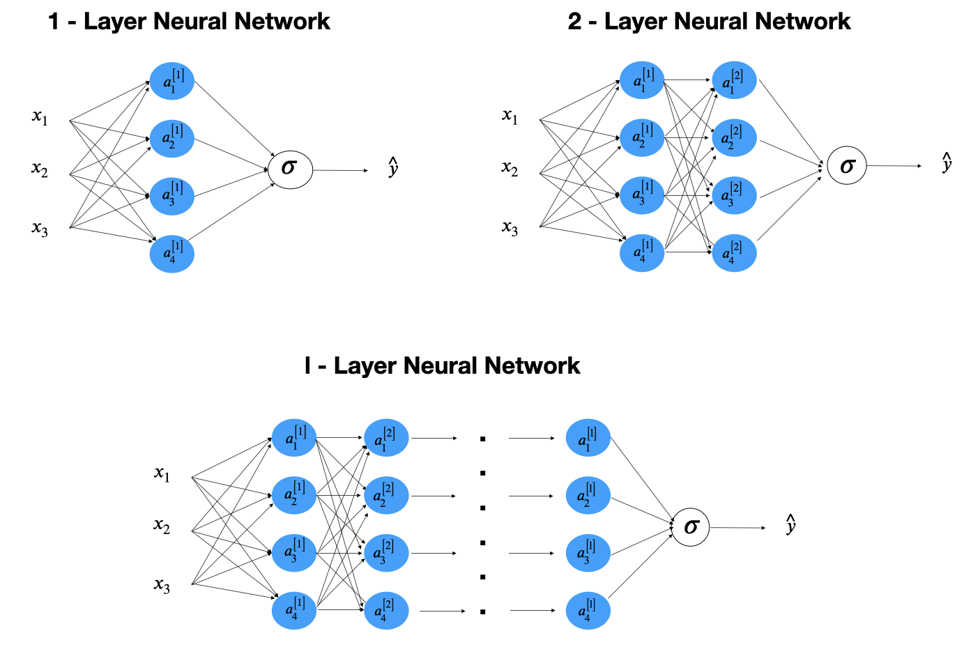
FIGURE 12.1: Feedforward Neural Network
Let’s look at a simple one-hidden-layer neural network (figure 12.2). First only consider one sample. From left to right, there is an input layer with 3 features (\(x_1, x_2, x_3\)), a hidden layer with four neurons and an output later to produce a prediction \(\hat{y}\).
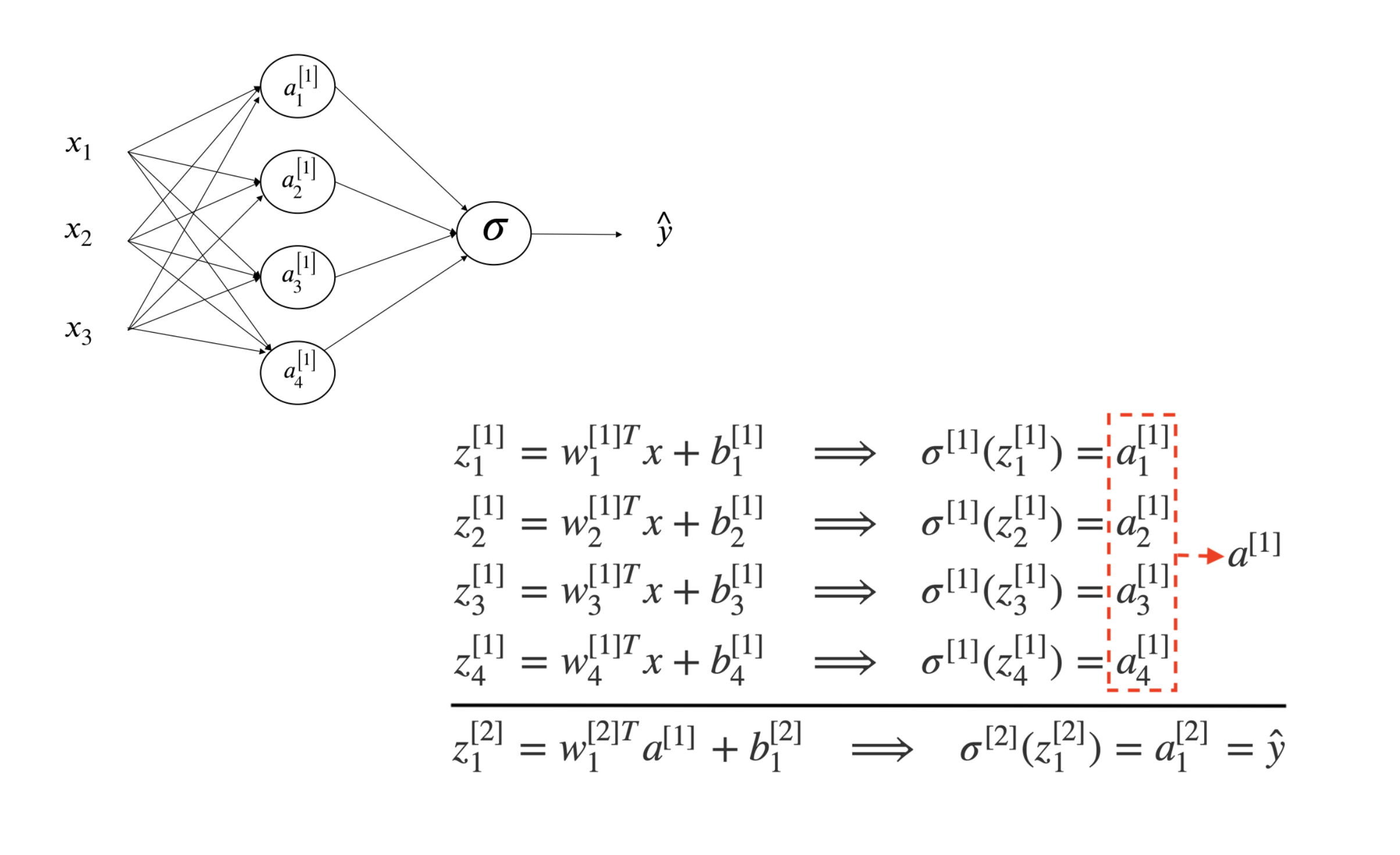
FIGURE 12.2: 1-layer Neural Network
From input to the first hidden layer
Each inactivated neuron on the first layer is a linear transformation of the input vector \(x\). For example, \(z^{[1]}_1 = w^{[1]T}_1x^{(i)} + b_1^{[1]}\) is the first inactivated neuron for hidden layer one. We use superscript [l] to denote a quantity associated with the \(l^{th}\) layer and the subscript i to denote the \(i^{th}\) entry of a vector (a neuron or feature). Here \(w^{[1]}\) and \(b_1^{[1]}\) are the weight and bias parameters for layer 1. \(w^{[1]}\) is a \(4 \times 1\) vector and hence \(w^{[1]T}_1x^{(i)}\) is a linear combination of the four input features. Then use a sigmoid function \(\sigma(\cdot)\) to activate the neuron \(z^{[1]}_1\) to get \(a^{[1]}_1\).
From the first hidden layer to the output
Next, do a linear combination of the activated neurons from the first layer to get inactivated output, \(z^{[2]}_1\). And then activate the neuron to get the predicted output \(\hat{y}\). The parameters to estimate in this step are \(w^{[2]}\) and \(b_1^{[2]}\).
If you fully write out the process, it is the bottom right of figure 12.2. When you implement a neural network, you need to do similar calculation four times to get the activated neurons in the first hidden layer. Doing this with a for loop is inefficient. So people vectorize the four equations. Take an input and compute the corresponding \(z\) and \(a\) as a vector. You can vectorize each step and get the following representation:
\[\begin{array}{cc} z^{[1]}=W^{[1]}x+b^{[1]} & \ \ \sigma^{[1]}(z^{[1]})=a^{[1]}\\ z^{[2]}=W^{[2]}a^{[1]}+b^{[2]} & \ \ \ \ \ \sigma^{[2]}(z^{[2]})=a^{[2]}=\hat{y} \end{array}\]
\(b^{[1]}\) is the column vector of the four bias parameters shown above. \(z^{[1]}\) is a column vector of the four non-active neurons. When you apply an activation function to a matrix or vector, you apply it element-wise. \(W^{[1]}\) is the matrix by stacking the four row-vectors:
\[W^{[1]}=\left[\begin{array}{c} w_{1}^{[1]T}\\ w_{2}^{[1]T}\\ w_{3}^{[1]T}\\ w_{4}^{[1]T} \end{array}\right]\]
So if you have one sample, you can go through the above forward propagation process to calculate the output \(\hat{y}\) for that sample. If you have \(m\) training samples, you need to repeat this process each of the \(m\) samples. We use superscript (i) to denote a quantity associated with \(i^{th}\) sample. You need to do the same calculation for all \(m\) samples.
For i = 1 to m, do:
\[\begin{array}{cc} z^{[1](i)}=W^{[1]}x^{(i)}+b^{[1]} & \ \ \sigma^{[1]}(z^{[1](i)})=a^{[1](i)}\\ z^{[2](i)}=W^{[2]}a^{[1](i)}+b^{[2]} & \ \ \ \ \ \sigma^{[2]}(z^{[2](i)})=a^{[2](i)}=\hat{y}^{(i)} \end{array}\]
Recall that we defined the matrix X to be equal to our training samples stacked up as column vectors in equation (12.1). We do a similar thing here to stack vectors with the superscript (i) together across \(m\) samples. This way, the neural network computes the outputs on all the samples on at the same time:
\[\begin{array}{cc} Z^{[1]}=W^{[1]}X+b^{[1]} & \ \ \sigma^{[1]}(Z^{[1]})=A^{[1]}\\ Z^{[2]}=W^{[2]}A^{[1]}+b^{[2]} & \ \ \ \ \ \sigma^{[2]}(Z^{[2]})=A^{[2]}=\hat{Y} \end{array}\]
where \[X=\left[\begin{array}{cccc} | & | & & |\\ x^{(1)} & x^{(1)} & \cdots & x^{(m)}\\ | & | & & | \end{array}\right],\]
\[A^{[l]}=\left[\begin{array}{cccc} | & | & & |\\ a^{[l](1)} & a^{[l](1)} & \cdots & a^{[l](m)}\\ | & | & & | \end{array}\right]_{l=1\ or\ 2},\]
\[Z^{[l]}=\left[\begin{array}{cccc} | & | & & |\\ z^{[l](1)} & z^{[l](1)} & \cdots & z^{[l](m)}\\ | & | & & | \end{array}\right]_{l=1\ or\ 2}\]
You can add layers like this to get a deeper neural network as shown in the bottom right of figure 12.1.
12.1.4 Activation Function
- Sigmoid and Softmax Function
We have used the sigmoid (or logistic) activation function. The function is S-shape with an output value between 0 to 1. Therefore it is used as the output layer activation function to predict the probability when the response \(y\) is binary. However, it is rarely used as an intermediate layer activation function. One of the main reasons is that when \(z\) is away from 0, then the derivative of the function drops fast which slows down the optimization process through gradient descent. Even with the fact that it is differentiable provides some convenience, the decreasing slope can cause a neural network to get stuck at the training time.

FIGURE 12.3: Sigmoid Function
When the output has more than 2 categories, people use softmax function as the output layer activation function.
\[\begin{equation} f_i(\mathbf{z}) = \frac{e^{z_i}}{\Sigma_{j=1}^{J} e^{z_j} } \tag{12.3} \end{equation}\]
where \(\mathbf{z}\) is a vector.
- Hyperbolic Tangent Function (tanh)
Another activation function with a similar S-shape is the hyperbolic tangent function. It often works better than the sigmoid function as the intermediate layer.
\[\begin{equation} tanh(z) = \frac{e^{z} - e^{-z}}{e^{z} + e^{-z}} \tag{12.4} \end{equation}\]

FIGURE 12.4: Hyperbolic Tangent Function
The tanh function crosses point (0, 0) and the value of the function is between 1 and -1 which makes the mean of the activated neurons closer to 0. The sigmoid function doesn’t have that property. When you preprocess the training input data, you sometimes center the data so that the mean is 0. The tanh function is doing that data processing in some way which makes learning for the next layer a little easier. This activation function is used a lot in the recurrent neural networks where you want to polarize the results.
- Rectified Linear Unit (ReLU) Function
The most popular activation function is the Rectified Linear Unit (ReLU) function. It is a piecewise function, or a half rectified function:
\[\begin{equation} R(z) = max(0, z) \tag{12.5} \end{equation}\]
The derivative is 1 when z is positive and 0 when z is negative. You can define the derivative as either 0 or 1 when z is 0.

FIGURE 12.5: Rectified Linear Unit Function
The advantage of the ReLU is that when z is positive, the derivative doesn’t vanish as z getting larger. So it leads to faster computation than sigmoid or tanh. It is non-linear with an unconstrained response. However, the disadvantage is that when z is negative, the derivative is 0. It may not map the negative values appropriately. In practice, this doesn’t cause too much trouble but there is another version of ReLu called leaky ReLu that attempts to solve the dying ReLU problem. The leaky ReLu is
\[R(z)_{Leaky}=\begin{cases} \begin{array}{c} z\\ az \end{array} & \begin{array}{c} z\geq0\\ z<0 \end{array}\end{cases}\]
Instead of being 0 when z is negative, it adds a slight slope such as \(a=0.01\) as shown in figure 12.6.

FIGURE 12.6: Rectified Linear Unit Function
You may notice that all activation functions are non-linear. Since the composition of two linear functions is still linear, using a linear activation function doesn’t help to capture more information. That is why you don’t see people use a linear activation function in the intermediate layer. One exception is when the output \(y\) is continuous, you may use linear activation function at the output layer. To sum up, for intermediate layers:
- ReLU is usually a good choice. If you don’t know what to choose, then start with ReLU. Leaky ReLu usually works better than the ReLU but it is not used as much in practice. Either one works fine. Also, people usually use a = 0.01 as the slope for leaky ReLU. You can try different parameters but most of the people a = 0.01.
- tanh is used sometimes especially in recurrent neural network. But you nearly never see people use sigmoid function as intermediate layer activation function.
For the output layer:
- When it is binary classification, use sigmoid with binary cross-entropy as loss function.
- When there are multiple classes, use softmax function with categorical cross-entropy as loss function.
- When the response is continuous, use identity function (i.e. y = x).
12.1.5 Optimization
So far, we have introduced the core components of deep learning architecture, layer, weight, activation function, and loss function. With the architecture in place, we need to determine how to update the network based on a loss function (a.k.a. objective function). In this section, we will look at variants of optimization algorithms that will improve the training speed.
12.1.5.1 Batch, Mini-batch, Stochastic Gradient Descent
Stochastic Gradient Descent (SGD) updates model parameters one sample each time. We showed the SGD for logistic regression across \(m\) samples in section 12.1.1. If you process the entire training set each time to calculate the gradient, it is Batch Gradient Descent (BGD). The vector representation section 12.1.3 using all \(m\) is an example of BGD.
In deep learning applications, the training set is often huge, with hundreds of thousands or millions of samples. If processing all the samples can only lead to one step of gradient descent, it could be slow. An intuitive way to improve the algorithm is to make some progress before finishing the entire data set. In particular, split up the training set into smaller subsets and fit the model using one subset each time. The subsets are mini-batches. Mini-batch Gradient Descent (MGD) is to split the training set to be smaller mini-batches. For example, if the mini-batch size is 1000, the algorithm will process 1000 samples each time, calculate the gradient and update the parameters. Then it moves on to the next mini-batch set until it goes through the whole training set. We call it one pass through training set using mini-batch gradient descent or one epoch. Epoch is a common keyword in deep learning, which means a single pass through the training set. If the training set has 60,000 samples, one epoch leads to 60 gradient descent steps. Then it will start over and take another pass through the training set. It means one more decision to make, the optimal number of epochs. It is decided by looking at the trends of performance metrics on a holdout set of training data. We discussed the data splitting and sampling in section 7.2. People often use a single holdout set to tune the model in deep learning. But it is important to use a big enough holdout set to give high confidence in your model’s overall performance. Then you can evaluate the chosen model on your test set that is not used in the training process. MGD is what everyone in deep learning uses when training on a large data set.
\[\begin{array}{ccc} x= & [\underbrace{x^{(1)},x^{(2)},\cdots,x^{(1000)}}/ & \cdots/\cdots x^{(m)}]\\ (n_{x},m) & mini-batch\ 1 \end{array}\]
\[\begin{array}{ccc} y= & [\underbrace{y^{(1)},y^{(2)},\cdots,y^{(1000)}}/ & \cdots/\cdots y^{(m)}]\\ (1,m) & mini-batch\ 1 \end{array}\]
- Mini-batch size = m: batch gradient descent, too long per iteration
- Mini-batch size = 1: stochastic gradient descent, lose speed from vectorization
- Mini-batch size in between: mini-batch gradient descent, make progress without processing all training set, typical batch sizes are \(2^6=64\), \(2^7=128\), \(2^8=256\), \(2^9=512\)
12.1.5.2 Optimization Algorithms
In the history of deep learning, researchers proposed different optimization algorithms and showed that they worked well in a specific scenario. But the optimization algorithms didn’t generalize well to a wide range of neural networks. So you will need to try different optimizers in your application. We will introduce three commonly used optimizers here, and they are all based on something called exponentially weighted averages. To understand the intuition behind it, let’s look at a hypothetical example shown in figure 12.7.
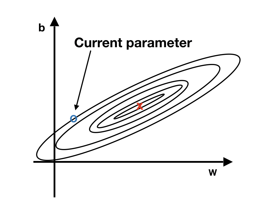
FIGURE 12.7: The intuition behind the weighted average gradient
We have two parameters, b and w. The blue dot represents the current parameter value, and the red point is the optimum value we want to reach. The current value is close to the target vertically but far away horizontally. In this situation, we hope to have slower learning on b and faster learning on w. A way to adjust is to use the average of the gradients from different iterations instead of the current iteration to update the parameter. Vertically, since the current value is close to the target value of parameter b, the gradient of b is likely to jump between positive and negative values. The average tends to cancel out the positive and negative derivatives along the vertical direction and slow down the oscillations. Horizontally, since it is still further away from the target value of parameter w, all the gradients are likely pointing in the same direction. Using an average won’t have too much impact there. That is the fundamental idea behind many different optimizers: adjust the learning rate using a weighted average of various iterations’ gradients.
Exponentially Weighted Averages
Before we get to more sophisticated optimization algorithms that implement this idea, let’s first introduce the basic weighted moving average framework.
Suppose we have the following 100 days’ temperature data:
\[ \theta_{1}=49F, \theta_{2}=53F, \dots, \theta_{99}=70F, \theta_{100}=69F\] The weighted average is defined as:
\[V_t = \beta V_{t-1}+(1-\beta)\theta_t\] And we have:
\[ \begin{array}{c} V_{0}=0\\ V_{1}=\beta V_1 + (1-\beta)\theta_1\\ V_2=\beta V_1 + (1-\beta)\theta_2\\ \vdots \\ V_{100}= \beta V_{99} + (1-\beta)\theta_{100} \end{array}\]
For example, for \(\beta=0.95\):
\[\begin{array}{c} V_{0}=0 \\ V_{1}=0.05\theta_{1} \\ V_{2}=0.0475\theta_{1}+0.05\theta_{2} \end{array} \\ ......\]
The black line in the left plot of figure 12.8 is the exponentially weighted averages of simulated temperature data with \(\beta = 0.95\). \(V_t\) is approximately average over the previous \(\frac{1}{1-\beta}\) days. So \(\beta = 0.95\) approximates a 20 days’ average. The red line corresponds to \(\beta = 0.8\), which approximates 5 days’ average. As \(\beta\) increases, it averages over a larger window of the previous values, and hence the curve gets smoother. A larger \(\beta\) also means that it gives the current value \(\theta_t\) less weight (\(1-\beta\)), and the average adapts more slowly. It is easy to see from the plot that the averages at the beginning are more biased. The bias correction can help to achieve a better estimate:
\[V_t^{corrected} = \frac{V_t}{1-\beta^t}\]
\[V_{1}^{corrected}=\frac{V_{1}}{1-0.95}=\theta_{1}\]
\[V_{2}^{corrected}=\frac{V_{2}}{1-0.95^{2}}=0.4872\theta_{1}+0.5128\theta_{2}\]
For \(\beta = 0.95\), the origional \(V_2 = 0.0475\theta_{1}+0.05\theta_{2}\) which is a small fraction of both \(theta_1\) and \(theta_2\). That is why it starts so much lower with big bias. After correction, \(V_{2}^{corrected} = 0.4872\theta_{1}+0.5128\theta_{2}\) is a weighted average with two weights added up to 1 which revmoves the bias. Notice that as \(t\) increases, \(\beta^t\) converges to 0 and \(V^{corrected}\) converges to \(V^t\).
The following code simulates a set of temperature data and applies exponentially weighted average with and without correction using various \(\beta\) values (0.5, 0.8, 0.95).
# simulate the tempreture data
a = -30/3479
b = -120 * a
c = 3600 * a + 80

day = c(1:100)
theta = a * day^2 + b * day + c + runif(length(day), -5, 5)
theta = round(theta, 0)

par(mfrow=c(1,2))
plot(day, theta, cex = 0.5, pch = 3, ylim = c(0, 100),
     main = "Without Correction",
     xlab = "Days", ylab = "Tempreture")

beta1 = 0.95
beta2 = 0.8
beta3 = 0.5

exp_weight_avg = function(beta, theta) {
  v = rep(0, length(theta))

  for (i in 1:length(theta)) {
    if (i == 1) {
      v[i] = (1 - beta) * theta[i]
    } else {
      v[i] = beta * v[i - 1] + (1 - beta) * theta[i]
    }
  }
  return(v)
}

v1 = exp_weight_avg(beta = beta1, theta)
v2 = exp_weight_avg(beta = beta2, theta)
v3 = exp_weight_avg(beta = beta3, theta)

lines(day, v1, col = 1)
lines(day, v2, col = 2)
lines(day, v3, col = 3)
legend("bottomright",
       paste0(c("beta1=","beta2=","beta3="),
              c(beta1, beta2, beta3)), col = c(1:3),
       lty = 1)

exp_weight_avg_correct = function(beta, theta) {
  v = rep(0, length(theta))

  for (i in 1:length(theta)) {
    if (i == 1) {
      v[i] = (1 - beta) * theta[i]
    } else {
      v[i] = beta * v[i - 1] + (1 - beta) * theta[i]
    }
  }
  v = v/(1 - beta^c(1:length(v)))
  return(v)
}

v1_correct = exp_weight_avg_correct(beta = beta1, theta)
v2_correct = exp_weight_avg_correct(beta = beta2, theta)
v3_correct = exp_weight_avg_correct(beta = beta3, theta)

plot(day, theta, cex = 0.5, pch = 3, ylim = c(0,100),
     main = "With Correction",
     xlab = "Days", ylab = "")

lines(day, v1_correct, col = 4)
lines(day, v2_correct, col = 5)
lines(day, v3_correct, col = 6)
legend("bottomright",
       paste0(c("beta1=","beta2=","beta3="),
              c(beta1, beta2, beta3)),
       col = c(4:6), lty = 1)
FIGURE 12.8: Exponentially weighted averages with and without corrrection
How do we apply the exponentially weighted average to optimization? Instead of using the gradients (\(dw\) and \(db\)) to update the parameter, we use the gradients’ exponentially weighted average. There are various optimizers built on top of this idea. We will look at three optimizers, Momentum, Root Mean Square Propagation (RMSprop), and Adaptive Moment Estimation (Adam).
Momentum
The momentum algorithm uses the exponentially weighted average of gradients to update the parameters. On iteration t, compute dw, db using samples in one mini-batch and update the parameters as follows:
\[V_{dw} = \beta V_{dw}+(1-\beta)dw\]
\[V_{db} = \beta V_{db}+(1-\beta)db\]
\[w=w-\alpha V_{dw};\ \ b=b-\alpha V_{db}\]
The learning rate \(\alpha\) and weighted average parameter \(\beta\) are hyperparameters. The most common and robust choice is \(\beta = 0.9\). This algorithm does not use the bias correction because the average will warm up after a dozen iterations and no longer be biased. The momentum algorithm, in general, works better than the original gradient descent without any average.
Root Mean Square Propagation (RMSprop)
The Root Mean Square Propagation (RMSprop) is another algorithm that applies the idea of exponentially weighted average. On iteration t, compute \(dw\) and \(db\) using the current mini-batch. Instead of \(V\), it calculates the weighted average of the squared gradient descents. When \(dw\) and \(db\) are vectors, the squaring is an element-wise operation.
\[S_{dw}=\beta S_{dw} + (1-\beta)dw^2\]
\[S_{db}=\beta S_{db} + (1-\beta)db^2\]
Then, update the parameters as follows:
\[w = w - \alpha \frac{dw}{\sqrt{S_{dw}}};\ b=b-\alpha \frac{db}{\sqrt{S_{db}}}\]
The RMSprop algorithm divides the learning rate for a parameter by a weighted average of recent gradients’ magnitudes for that parameter. The goal is still to adjust the learning speed. Recall the example that illustrates the intuition behind it. When parameter b is close to its target value, we want to decrease the oscillations along the vertical direction.
Adaptive Moment Estimation (Adam)
The Adaptive Moment Estimation (Adam) algorithm is, in some way, a combination of momentum and RMSprop. On iteration t, compute dw, db using the current mini-batch. Then calculate both V and S using the gradient descents.
\[\begin{cases} \begin{array}{c} V_{dw}=\beta_{1}V_{dw}+(1-\beta_{1})dw\\ V_{db}=\beta_{1}V_{db}+(1-\beta_{1})db \end{array} & momantum\ update\ \beta_{1}\end{cases}\]
\[\begin{cases} \begin{array}{c} S_{dw}=\beta_{2}S_{dw}+(1-\beta_{2})dw^{2}\\ S_{db}=\beta_{2}S_{db}+(1-\beta_{2})db^{2} \end{array} & RMSprop\ update\ \beta_{2}\end{cases}\]
The Adam algorithm implements bias correction.
\[\begin{cases} \begin{array}{c} V_{dw}^{corrected}=\frac{V_{dw}}{1-\beta_{1}^{t}}\\ V_{db}^{corrected}=\frac{V_{db}}{1-\beta_{1}^{t}} \end{array}\end{cases};\ \ \begin{cases} \begin{array}{c} S_{dw}^{corrected}=\frac{S_{dw}}{1-\beta_{2}^{t}}\\ S_{db}^{corrected}=\frac{S_{db}}{1-\beta_{2}^{t}} \end{array}\end{cases}\]
And it updates the parameter using both corrected V and S. \(\epsilon\) here is a tiny positive number to make sure the denominator is larger than zero. The choice of \(\epsilon\) doesn’t matter much, and the inventors of the Adam algorithm recommended \(\epsilon = 10^{-8}\). For hyperparameter \(\beta_1\) and \(\beta_2\), the common settings are \(\beta_1 = 0.9\) and \(\beta_2 = 0.999\).
\[w=w-\alpha \frac{V_{dw}^{corrected}}{\sqrt{S_{dw}^{corrected}} +\epsilon};\ b=b-\alpha\frac{V_{db}^{corrected}}{\sqrt{S_{db}^{corrected}}+\epsilon}\]
12.1.6 Deal with Overfitting
The biggest problem for deep learning is overfitting. It happens when the model learns too much from the data. We discussed this in more detail in section 7.1. A common way to diagnose the problem is to use cross-validation (section 7.2). You can recognize the problem when the model fits great on the training data but gives poor predictions on the testing data. One way to prevent the model from over learning the data is to limit model complexity. There are several approaches to that.
12.1.6.1 Regularization
For logistic regression, we can add a penalty term:
\[\underset{w,b}{min}J(w,b)= \frac{1}{m} \Sigma_{i=1}^{m}L(\hat{y}^{(i)}, y^{(i)}) + penalty\]
Common penalties are L1 or L2 as follows:
\[L_2\ penalty=\frac{\lambda}{2m}\parallel w \parallel_2^2 = \frac{\lambda}{2m}\Sigma_{i=1}^{n_x}w_i^2\]
\[L_1\ penalty = \frac{\lambda}{m}\Sigma_{i=1}^{n_x}|w|\]
For neural network,
\[J(w^{[1]},b^{[1]},\dots,w^{[L]},b^{[L]})=\frac{1}{m}\Sigma_{i=1}^{m}L(\hat{y}^{(i)},y^{(i)}) + \frac{\lambda}{2}\Sigma_{l=1}^{L} \parallel w^{[l]} \parallel^2_F\]
where
\[\parallel w^{[l]} \parallel^2_F = \Sigma_{i=1}^{n^{[l]}}\Sigma_{j=1}^{n^{[l-1]}} (w^{[l]}_{ij})^2\]
Many people call it “Frobenius Norm” instead of L2-norm.
12.1.6.2 Dropout
Another powerful regularization technique is “dropout.” In chapter 11, we mentioned that the random forest model de-correlates the trees by randomly choosing a subset of features. Dropout uses a similar idea in the parameter estimation process.
It temporally freezes a randomly selected subset of nodes at a specific layer in the neural network during the optimization process to reduce overfitting. When applying dropout to a particular layer and mini-batch, we pre-set a percentage, for example, 30%, and randomly remove 30% of the layer’s nodes. The output from the 30% removed nodes will be zero. During backpropagation, we update the remaining parameters for a much-diminished network. We need to do the random drop out again for the next mini-batch.
To normalize the output with all nodes in this layer, we need to scale up the output accordingly to the same percentage to make sure the dropped-out nodes do not impact the overall signal. Please note, the dropout process will randomly turn-off different nodes for each mini-batch. Dropout is more efficient in reducing overfitting in deep learning than L1 or L2 regularizations.
12.1.7 Image Recognition Using FFNN
In this section, we will walk through a toy example of image classification problem using keras package. We use R in the section to illustrate the process and also provide the python notebook on the book website. Please check the keras R package website for the most recent development.
What is an image as data? You can consider a digital image as a set of points on 2-d or 3-d space. For a grey scale image, each point has a value between 0 to 255 which is considered as a pixel. Figure 12.9 shows an example of grayscale image. It is a set of pixels on 2-d space and each pixel has a value between 0 to 255. You can process the image as a 2-d array input if you use a Convolutional Neural Network (CNN). Or, you can vectorize the 2D array into 1D vector as the input for FFNN as shown in the figure.
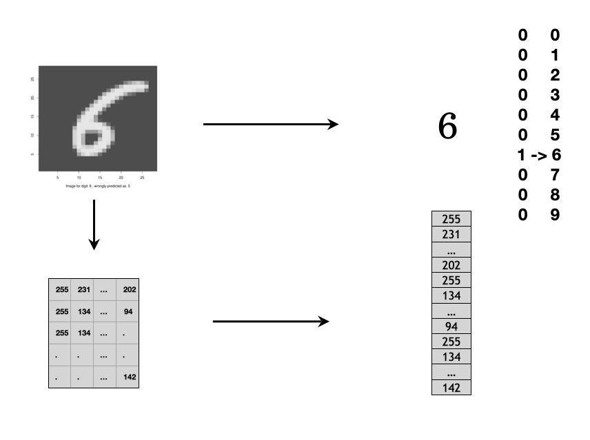
FIGURE 12.9: Grayscale image is a set of pixels on 2-d space. Each pixel has a value range from 0 to 255.
A color image is a set of pixels on 3-d space and each pixel has a value between 0 to 255 for a specfic color format. There are three 2-d panels which represent the color red, blue and green accordingly. Similarly, You can process the image as a 3-d array. Or you can vectorize the array as shown in figure 12.10.
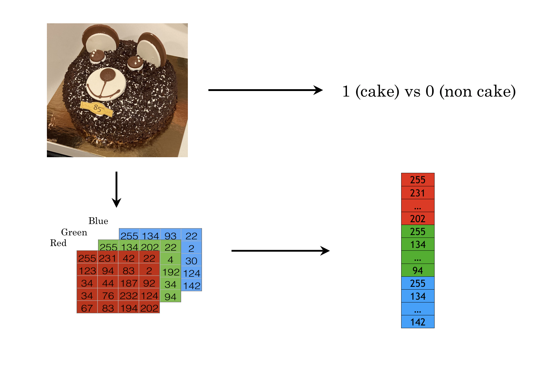
FIGURE 12.10: Color image is a set of pixels on 3-d space. Each pixel has a value range from 0 to 255.
Let’s look at how to use the keras R package for a toy example in deep learning with the handwritten digits image dataset (i.e. MNIST). keras has many dependent packages, so it takes a few minutes to install.
install.packages("keras")As keras is just an interface to popular deep learning frameworks, we have to install the deep learning backend. The default and recommended backend is TensorFlow. By calling install_keras(), it will install all the needed dependencies for TensorFlow.
library(keras)
install_keras()
You can run the code in this section in the Databrick community edition with R as the interface. Refer to section 4.3 for how to set up an account, create a notebook (R or Python) and start a cluster. For an audience with a statistical background, using a well-managed cloud environment has the following benefit:
- Minimum language barrier in coding for most statisticians
- Zero setups to save time using the cloud environment
- Get familiar with the current trend of cloud computing in the industrial context
You can also run the code on your local machine with R and the required Python packages (keras uses the Python TensorFlow backend engine). Different versions of Python may cause some errors when running install_keras(). Here are the things you could do when you encounter the Python backend issue in your local machine:
- Run
reticulate::py_config()to check the current Python configuration to see if anything needs to be changed. - By default,
install_keras()uses virtual environment~/.virtualenvs/r-reticulate. If you don’t know how to set the right environment, try to set the installation method as conda (install_keras(method = "conda")) - Refer to this document for more details on how to install
kerasand the TensorFlow backend.
Now we are all set to explore deep learning! As simple as three lines of R code, but there are quite a lot going on behind the scene. If you are using a cloud environment, you do not need to worry about these behind scene setup and maintenance.
We will use the widely used MNIST handwritten digit image dataset. More information about the dataset and benchmark results from various machine learning methods can be found at http://yann.lecun.com/exdb/mnist/ and https://en.wikipedia.org/wiki/MNIST_database.
This dataset is already included in the keras/TensorFlow installation and we can simply load the dataset as described in the following cell. It takes less than a minute to load the dataset.
mnist <- dataset_mnist()The data structure of the MNIST dataset is straight forward and well prepared for R, which has two pieces:
training set: x (i.e. features): 60000x28x28 tensor which corresponds to 60000 28x28 pixel greyscale images (i.e. all the values are integers between 0 and 255 in each 28x28 matrix), and y (i.e. responses): a length 60000 vector which contains the corresponding digits with integer values between 0 and 9.
testing set: same as the training set, but with only 10000 images and responses. The detailed structure for the dataset can be seen with
str(mnist)below.
str(mnist)List of 2
$ train:List of 2
..$ x: int [1:60000, 1:28, 1:28] 0 0 0 0 0 0 0 0 0 0 ...
..$ y: int [1:60000(1d)] 5 0 4 1 9 2 1 3 1 4 ...
$ test :List of 2
..$ x: int [1:10000, 1:28, 1:28] 0 0 0 0 0 0 0 0 0 0 ...
..$ y: int [1:10000(1d)] 7 2 1 0 4 1 4 9 5 9 ...Now we prepare the features (x) and the response variable (y) for both the training and testing dataset, and we can check the structure of the x_train and y_train using str() function.
x_train <- mnist$train$x
y_train <- mnist$train$y
x_test <- mnist$test$x
y_test <- mnist$test$y

str(x_train)
str(y_train)
int [1:60000, 1:28, 1:28] 0 0 0 0 0 0 0 0 0 0 ...
int [1:60000(1d)] 5 0 4 1 9 2 1 3 1 4 ...Now let’s plot a chosen 28x28 matrix as an image using R’s image() function. In R’s image() function, the way of showing an image is rotated 90 degree from the matrix representation. So there is additional steps to rearrange the matrix such that we can use image() function to show it in the actual orientation.
index_image = 28  ## change this index to see different image.
input_matrix <- x_train[index_image, 1:28, 1:28]
output_matrix <- apply(input_matrix, 2, rev)
output_matrix <- t(output_matrix)
image(1:28, 1:28, output_matrix, col = gray.colors(256),
    xlab = paste("Image for digit of: ", y_train[index_image]),
    ylab = "")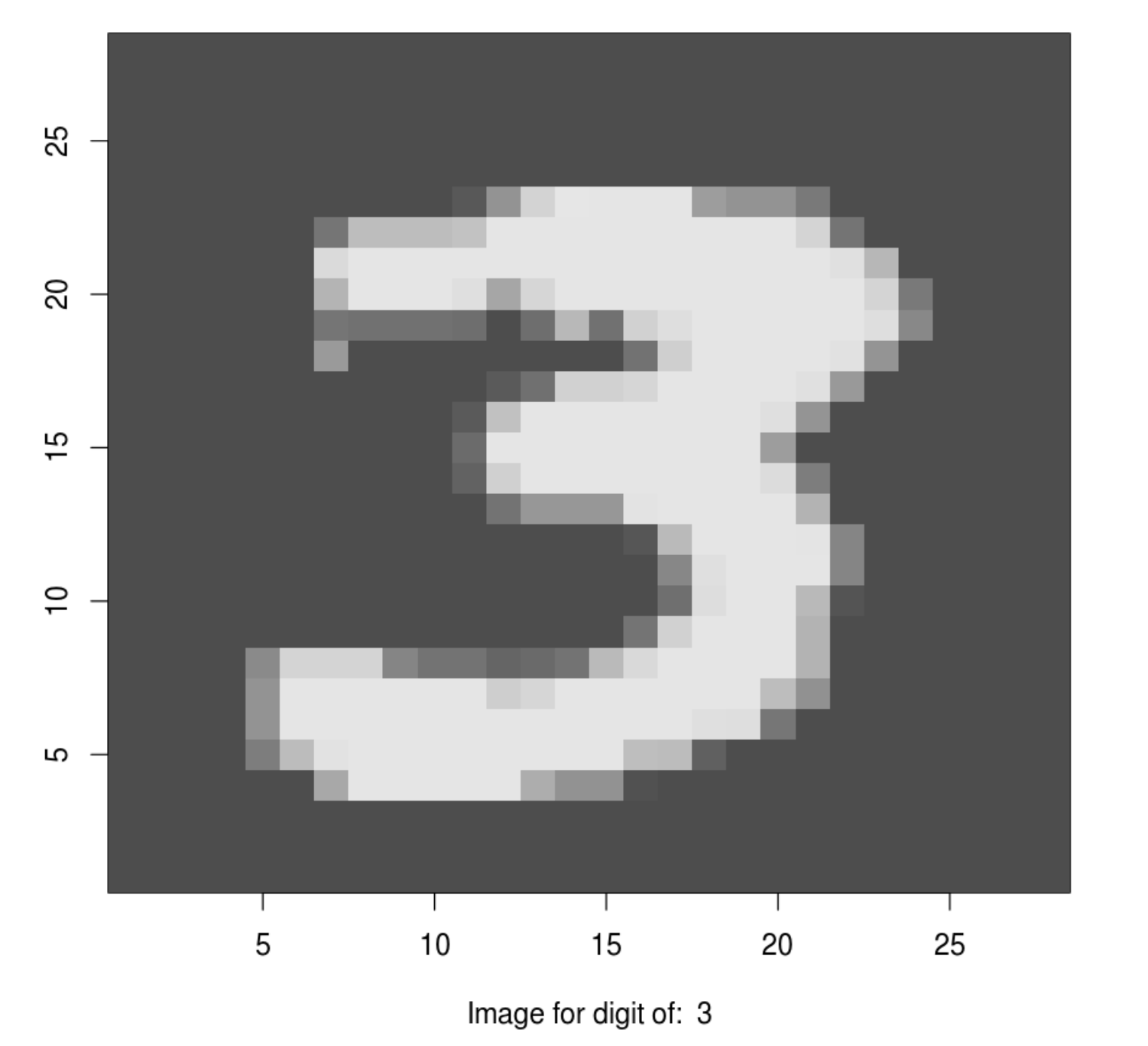
Here is the original 28x28 matrix for the above image:
dplyr::tibble(input_matrix)## # A tibble: 28 × 1
## input_matrix[,1] [,2] [,3] [,4] [,5] [,6] [,7] [,8] [,9] [,10] [,11]
## <int> <int> <int> <int> <int> <int> <int> <int> <int> <int> <int>
## 1 0 0 0 0 0 0 0 0 0 0 0
## 2 0 0 0 0 0 0 0 0 0 0 0
## 3 0 0 0 0 0 0 0 0 0 0 0
## 4 0 0 0 0 0 0 0 0 0 0 0
## 5 0 0 0 0 0 0 0 0 0 0 0
## 6 0 0 0 0 0 0 0 0 0 0 9
## # … with 22 more rows, and 1 more variable: input_matrix[12:28] <int>
...There are multiple deep learning methods to solve the handwritten digits problem and we will start from the simple and generic one, feedforward neural network (FFNN). FFNN contains a few fully connected layers and information is flowing from a front layer to a back layer without any feedback loop from the back layer to the front layer. It is the most common deep learning models to start with.
12.1.7.1 Data preprocessing
In this section, we will walk through the needed steps of data preprocessing. For the MNIST dataset that we just loaded, some preprocessing is already done. So we have a relatively “clean” data, but before we feed the data into FFNN, we still need to do some additional preparations.
First, for each digits, we have a scalar response and a 28x28 integer matrix with value between 0 and 255. To use the out of box DNN functions, for each response, all the features are one row of all features. For an image in MNIST dataet, the input for one response y is a 28x28 matrix, not a single row of many columns and we need to convet the 28x28 matrix into a single row by appending every row of the matrix to the first row using reshape() function.
In addition, we also need to scale all features to be between (0, 1) or (-1, 1) or close to (-1, 1) range. Scale or normalize every feature will improve numerical stability in the optimization procedure as there are a lot of parameters to be optimized.
We first reshape the 28x28 image for each digit (i.e each row) into 784 columns (i.e. features), and then rescale the value to be between 0 and 1 by dividing the original pixel value by 255, as described in the cell below.
# step 1: reshape
x_train <- array_reshape(x_train,
                         c(nrow(x_train), 784))
x_test <- array_reshape(x_test,
                        c(nrow(x_test), 784))

# step 2: rescale
x_train <- x_train / 255
x_test <- x_test / 255
And here is the structure of the reshaped and rescaled features for training and testing dataset. Now for each digit, there are 784 columns of features.
str(x_train)
str(x_test)
num [1:60000, 1:784] 0 0 0 0 0 0 0 0 0 0 ...
num [1:10000, 1:784] 0 0 0 0 0 0 0 0 0 0 ...In this example, though the response variable is an integer (i.e. the corresponding digits for an image), there is no order or rank for these integers and they are just an indication of one of the 10 categories. So we also convert the response variable y to be categorical.
y_train <- to_categorical(y_train, 10)
y_test <- to_categorical(y_test, 10)
str(y_train)
num [1:60000, 1:10] 0 1 0 0 0 0 0 0 0 0 ...12.1.7.2 Fit model
Now we are ready to fit the model. It is straight forward to build a deep neural network using keras. For this example, the number of input features is 784 (i.e. scaled value of each pixel in the 28x28 image) and the number of class for the output is 10 (i.e. one of the ten categories). So the input size for the first layer is 784 and the output size for the last layer is 10. And we can add any number of compatible layers in between.
In keras, it is easy to define a DNN model: (1) use keras_model_sequential() to initiate a model placeholder and all model structures are attached to this model object, (2) layers are added in sequence by calling the layer_dense() function, (3) add arbitrary layers to the model based on the sequence of calling layer_dense(). For a dense layer, all the nodes from the previous layer are connected with each and every node to the next layer. In layer_dense() function, we can define how many nodes in that layer through the units parameter. The activation function can be defined through the activation parameter. For the first layer, we also need to define the input features’ dimension through input_shape parameter. For our preprocessed MNIST dataset, there are 784 columns in the input data. A common way to reduce overfitting is to use the dropout method, which randomly drops a proportion of the nodes in a layer. We can define the dropout proportion through layer_dropout() function immediately after the layer_dense() function.
dnn_model <- keras_model_sequential()
dnn_model %>%
  layer_dense(units = 256, activation = 'relu', input_shape = c(784)) %>%
  layer_dropout(rate = 0.4) %>%
  layer_dense(units = 128, activation = 'relu') %>%
  layer_dropout(rate = 0.3) %>%
  layer_dense(units = 64, activation = 'relu') %>%
  layer_dropout(rate = 0.3) %>%
  layer_dense(units = 10, activation = 'softmax')
The above dnn_model has 4 layers with first layer 256 nodes, 2nd layer 128 nodes, 3rd layer 64 nodes, and last layer 10 nodes. The activation function for the first 3 layers is relu and the activation function for the last layer is softmax which is typical for classification problems. The model detail can be obtained through summary() function. The number of parameter of each layer can be calculated as: (number of input features +1) times (numbe of nodes in the layer). For example, the first layer has (784+1)x256=200960 parameters; the 2nd layer has (256+1)x128=32896 parameters. Please note, dropout only randomly drop certain proportion of parameters for each batch, it will not reduce the number of parameters in the model. The total number of parameters for the dnn_model we just defined has 242762 parameters to be estimated.
summary(dnn_model)________________________________________________________________________________
Layer (type) Output Shape Param #
================================================================================
dense_1 (Dense) (None, 256) 200960
________________________________________________________________________________
dropout_1 (Dropout) (None, 256) 0
________________________________________________________________________________
dense_2 (Dense) (None, 128) 32896
________________________________________________________________________________
dropout_2 (Dropout) (None, 128) 0
________________________________________________________________________________
dense_3 (Dense) (None, 64) 8256
________________________________________________________________________________
dropout_3 (Dropout) (None, 64) 0
________________________________________________________________________________
dense_4 (Dense) (None, 10) 650
================================================================================
Total params: 242,762
Trainable params: 242,762
Non-trainable params: 0
________________________________________________________________________________Once a model is defined, we need to compile the model with a few other hyper-parameters including (1) loss function, (2) optimizer, and (3) performance metrics. For multi-class classification problems, people usually use the categorical_crossentropy loss function and optimizer_rmsprop() as the optimizer which performs batch gradient descent.
dnn_model %>% compile(
  loss = 'categorical_crossentropy',
  optimizer = optimizer_rmsprop(),
  metrics = c('accuracy')
)
Now we can feed data (x and y) into the neural network that we just built to estimate all the parameters in the model. Here we define three hyperparameters: epochs, batch_size, and validation_split, for this model. It just takes a couple of minutes to finish.
dnn_history <- dnn_model %>% fit(
  x_train, y_train,
  epochs = 15, batch_size = 128,
  validation_split = 0.2
)
There is some useful information stored in the output object dnn_history and the details can be shown by using str(). We can plot the training and validation accuracy and loss as function of epoch by simply calling plot(dnn_history).
str(dnn_history)List of 2
$ params :List of 8
..$ metrics : chr [1:4] "loss" "acc" "val_loss" "val_acc"
..$ epochs : int 15
..$ steps : NULL
..$ do_validation : logi TRUE
..$ samples : int 48000
..$ batch_size : int 128
..$ verbose : int 1
..$ validation_samples: int 12000
$ metrics:List of 4
..$ acc : num [1:15] 0.83 0.929 0.945 0.954 0.959 ...
..$ loss : num [1:15] 0.559 0.254 0.195 0.165 0.148 ...
..$ val_acc : num [1:15] 0.946 0.961 0.967 0.969 0.973 ...
..$ val_loss: num [1:15] 0.182 0.137 0.122 0.113 0.104 ...
- attr(*, "class")= chr "keras_training_history"plot(dnn_history)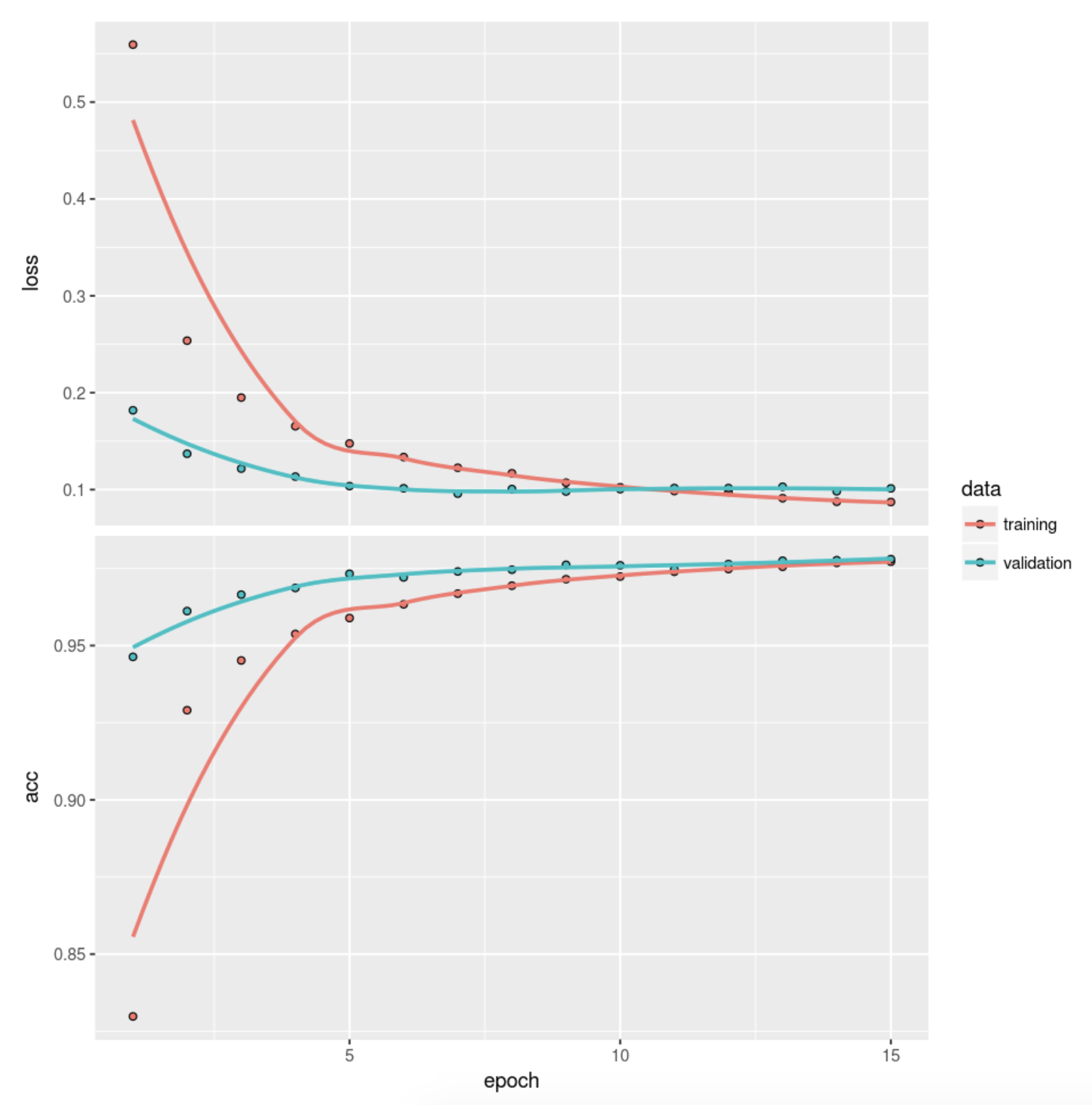
12.1.7.3 Prediction
dnn_model %>% evaluate(x_test, y_test)## loss accuracy
## 0.09035096 0.98100007dnn_pred <- dnn_model %>%
predict(x_test) %>%
k_argmax()
head(dnn_pred)tf.Tensor([7 2 1 0 4 1], shape=(6,), dtype=int64)Let’s check a few misclassified images. A number of misclassified images can be found using the following code. And we can plot these misclassified images to see whether a human can correctly read it out.
## Convert tf.tensor to array
dnn_pred <- as.array(dnn_pred)
## total number of mis-classcified images
sum(dnn_pred != mnist$test$y)
[1] 190missed_image = mnist$test$x[dnn_pred != mnist$test$y,,]
missed_digit = mnist$test$y[dnn_pred != mnist$test$y]
missed_pred = dnn_pred[dnn_pred != mnist$test$y]
index_image = 34
## change this index to see different image.
input_matrix <- missed_image[index_image,1:28,1:28]
output_matrix <- apply(input_matrix, 2, rev)
output_matrix <- t(output_matrix)
image(1:28, 1:28, output_matrix, col = gray.colors(256),
xlab = paste("Image for digit ", missed_digit[index_image],
", wrongly predicted as ", missed_pred[index_image]),
ylab = "")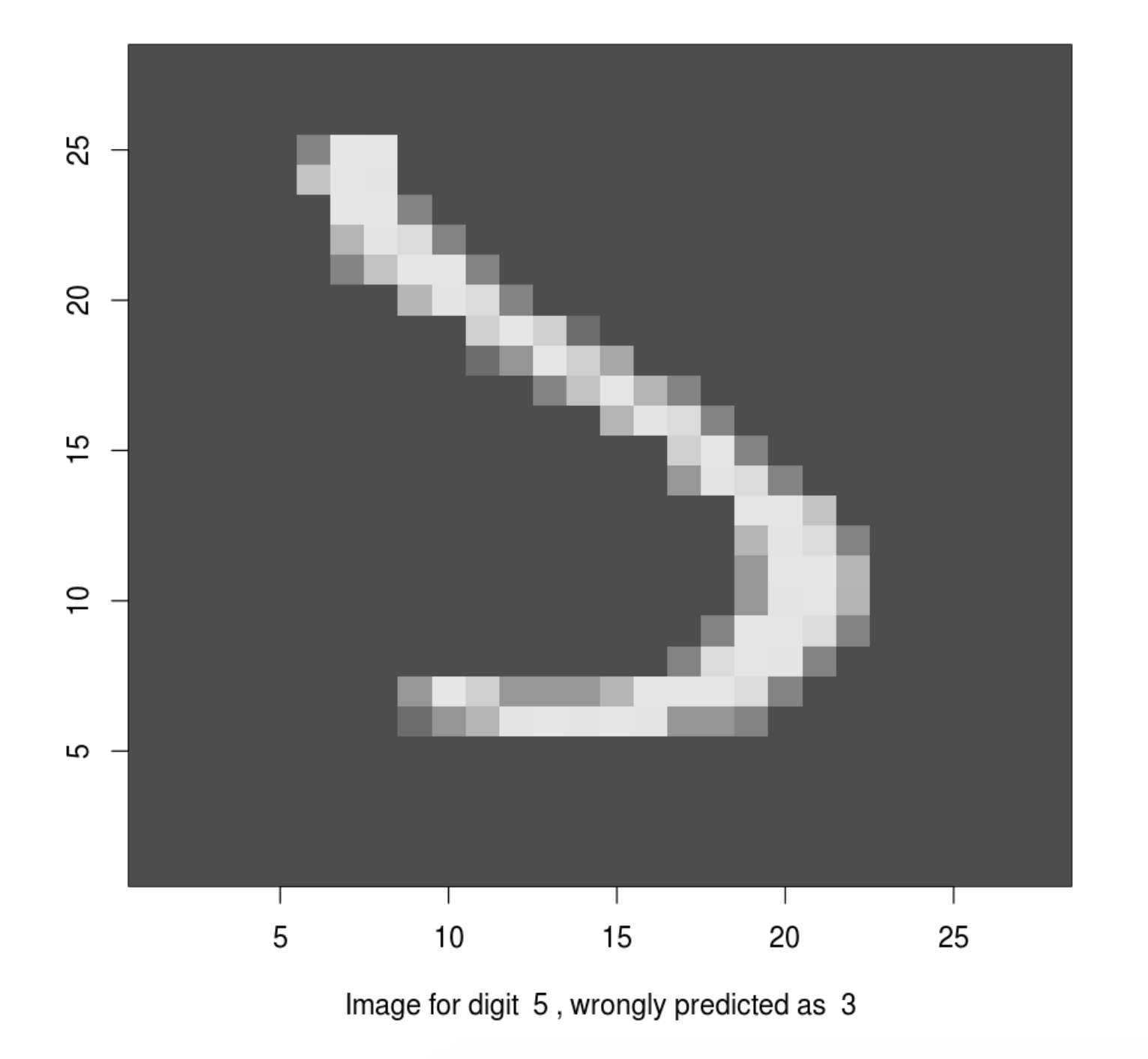
Now we finish this simple tutorial of using deep neural networks for handwritten digit recognition using the MNIST dataset. We illustrate how to reshape the original data into the right format and scaling; how to define a deep neural network with arbitrary number of layers; how to choose activation function, optimizer, and loss function; how to use dropout to limit overfitting; how to setup hyperparameters; and how to fit the model and using a fitted model to predict. Finally, we illustrate how to plot the accuracy/loss as functions of the epoch. It shows the end-to-end cycle of how to fit a deep neural network model.
On the other hand, the image can be better dealt with Convolutional Neural Network (CNN) and we are going to walk through the exact same problem using CNN in the next section.