7.2 Data Splitting and Resampling
Highly adaptable models can model complex relationships. However, they tend to overfit, which leads to a poor prediction by learning too much from the current sample set. Those models are susceptible to the specific sample set used to fit them. The model prediction may be off when future data is unlike past data. Conversely, a simple model, such as ordinary linear regression, tends to underfit, leading to a poor prediction by learning too little from the data. It systematically over-predicts or under-predicts the data regardless of how well future data resemble past data.
Model evaluation is essential to assess the efficacy of a model. A modeler needs to understand how a model fits the existing data and how it would work on future data. Also, trying multiple models and comparing them is always a good practice. All these need data splitting and resampling.
7.2.1 Data Splitting
Data splitting is to put part of the data aside as an evaluation set (or hold-outs, out-of-bag samples) and use the rest for model tuning. Training samples are also called in-sample. Model performance metrics evaluated using in-sample are retrodictive, not predictive.
Traditional business intelligence usually handles data description. Answer simple questions by querying and summarizing the data, such as:
- What are the monthly sales of a product in 2020?
- What is the number of site visits in the past month?
- What is the sales difference in 2021 for two different product designs?
There is no need to go through the tedious process of splitting the data, tuning, and evaluating a model to answer questions of this kind.
Some models have hyperparameters (aka. tuning parameters) not derived by training the model, such as the penalty parameter in lasso, the number of trees in a random forest, and the learning rate in deep learning. They often control the model’s process, and no analytical formula is available to calculate the optimized value. A poor choice can result in over-fitting, under-fitting, or optimization failure. A standard approach to searching for the best tuning parameters is through cross-validation, which is a data resampling approach.
To get a reasonable performance precision based on a single test set, the size of the test set may need to be large. So a conventional approach is to use a subset of samples to fit the model and use the rest to evaluate model performance. This process will repeat multiple times to get a performance profile. In that sense, resampling is based on splitting. The general steps are:
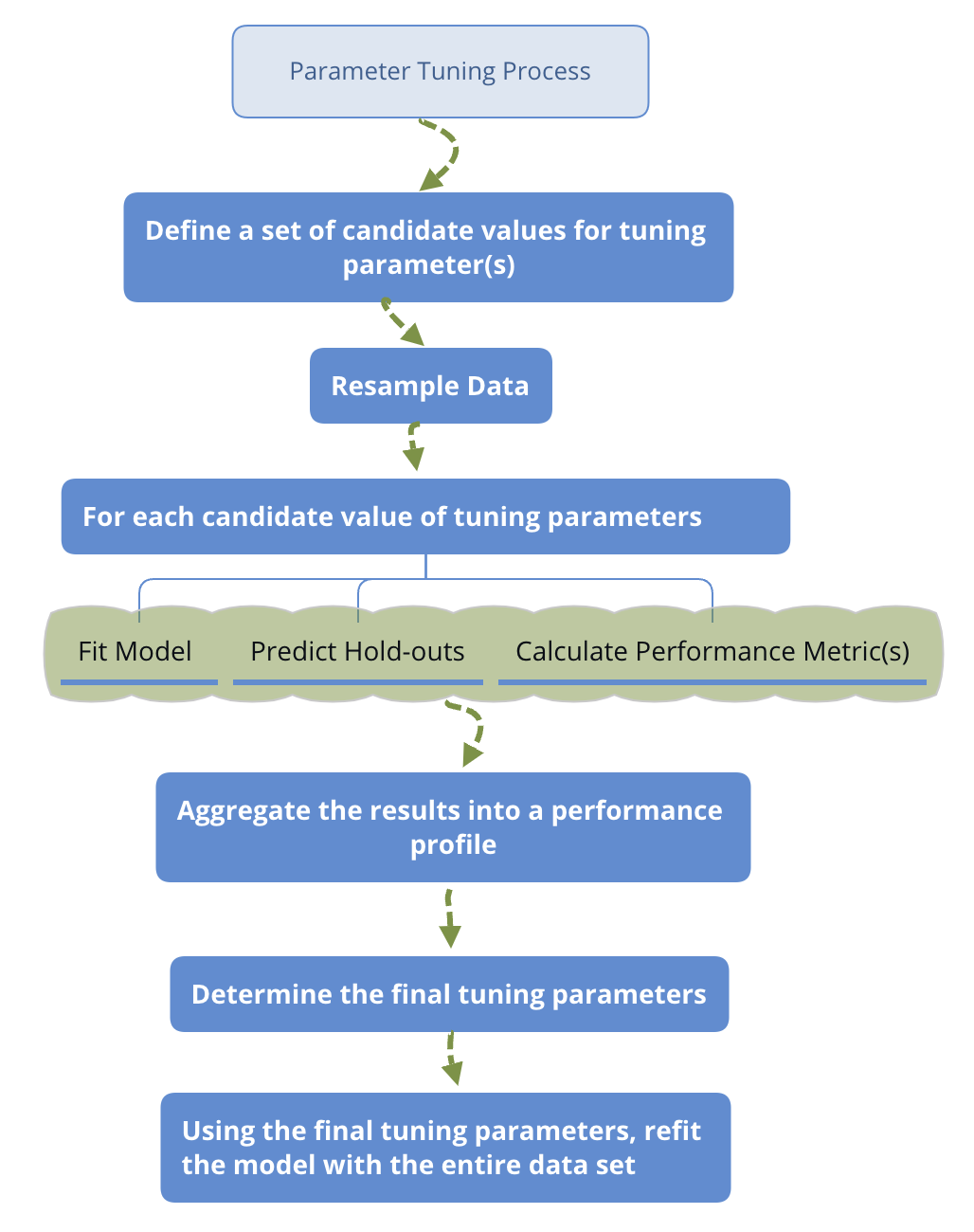
Parameter Tuning Process
The above is an outline of the general procedure to tune parameters. Now let’s focus on the critical part of the process: data splitting. Ideally, we should evaluate the model using samples not used to build or fine-tune the model. So it provides an unbiased sense of model effectiveness. When the sample size is large, it is a good practice to set aside part of the samples to evaluate the final model. People use training data to indicate the sample set used to fit the model. Use testing data to tune hyperparameters and validation data to evaluate performance and compare different models.
Let’s focus on data splitting in the model tuning process, where we split data into training and testing sets.
The first decision is the proportion of data in the test set. There are two factors to consider here: (1) sample size; (2) computation intensity. Suppose the sample size is large enough, which is the most common situation according to my experience. In that case, you can try using 20%, 30%, and 40% of the data as the test set and see which works best. If the model is computationally intense, you may consider starting from a smaller subset to train the model and hence have a higher portion of data in the test set. You may need to increase the training set depending on how it performs. If the sample size is small, you can use cross-validation or bootstrap, which is the topic of the next section.
The next is to decide which samples are in the test set. There is a desire to make the training and test sets as similar as possible. A simple way is to split data randomly, which does not control for any data attributes. However, sometimes we may want to ensure that training and testing data have a similar outcome distribution. For example, suppose you want to predict the likelihood of customer retention. In that case, you want two data sets with a similar percentage of retained customers.
There are three main ways to split the data that account for the similarity of resulted data sets. We will describe the three approaches using the clothing company’s customer data as examples.
- Split data according to the outcome variable
Assume the outcome variable is customer segment (column segment), and we decide to use 80% as training and 20% as testing. The goal is to make the proportions of the categories in the two sets as similar as possible. The createDataPartition() function in caret will return a balanced splitting based on assigned variable.
# load data
sim.dat <- read.csv("http://bit.ly/2P5gTw4")
library(caret)
# set random seed to make sure reproducibility
set.seed(3456)
trainIndex <- createDataPartition(sim.dat$segment,
                                  p = 0.8,
                                  list = FALSE,
                                  times = 1)
head(trainIndex)
## Resample1
## [1,] 1
## [2,] 2
## [3,] 3
## [4,] 4
## [5,] 6
## [6,] 7The list = FALSE in the call to createDataPartition is to return a data frame. The times = 1 tells R how many times you want to split the data. Here we only do it once, but you can repeat the splitting multiple times. In that case, the function will return multiple vectors indicating the rows to training/test. You can set times = 2 and rerun the above code to see the result. Then we can use the returned indicator vector trainIndex to get training and test sets:
# get training set
datTrain <- sim.dat[trainIndex, ]
# get test set
datTest <- sim.dat[-trainIndex, ]
According to the setting, there are 800 samples in the training set and 200 in the testing set. Let’s check the distribution of the two groups:
datTrain %>%
  dplyr::group_by(segment) %>%
  dplyr::summarise(count = n(),
            percentage = round(length(segment)/nrow(datTrain), 2))
## # A tibble: 4 × 3
## segment count percentage
## <chr> <int> <dbl>
## 1 Conspicuous 160 0.2
## 2 Price 200 0.25
## 3 Quality 160 0.2
## 4 Style 280 0.35datTest %>%
dplyr::group_by(segment) %>%
dplyr::summarise(count = n(),
percentage = round(length(segment)/nrow(datTest), 2))## # A tibble: 4 × 3
## segment count percentage
## <chr> <int> <dbl>
## 1 Conspicuous 40 0.2
## 2 Price 50 0.25
## 3 Quality 40 0.2
## 4 Style 70 0.35The percentages are the same for these two sets. In practice, it is possible that the distributions are not identical but should be close.
- Divide data according to predictors
An alternative way is to split data based on the predictors. The goal is to get a diverse subset from a dataset to represent the sample. In other words, we need an algorithm to identify the \(n\) most diverse samples from a dataset with size \(N\). However, the task is generally infeasible for non-trivial values of \(n\) and \(N\) (Willett 2004). And hence practicable approaches to dissimilarity-based selection involve approximate methods that are sub-optimal. A major class of algorithms split the data on maximum dissimilarity sampling. The process starts from:
- Initialize a single sample as starting test set
- Calculate the dissimilarity between this initial sample and each remaining samples in the dataset
- Add the most dissimilar unallocated sample to the test set
To move forward, we need to define the dissimilarity between groups. Each definition results in a different version of the algorithm and hence a different subset. It is the same problem as in hierarchical clustering where you need to define a way to measure the distance between clusters. The possible approaches are to use minimum, maximum, sum of all distances, the average of all distances, etc. Unfortunately, there is not a single best choice, and you may have to try multiple methods and check the resulted sample sets. R users can implement the algorithm using maxDissim() function from caret package. The obj argument is to set the definition of dissimilarity. Refer to the help documentation for more details (?maxDissim).
Let’s use two variables (age and income) from the customer data as an example to illustrate how it works in R and compare maximum dissimilarity sampling with random sampling.
library(lattice)
# select variables
testing <- subset(sim.dat, select = c("age", "income"))
Random select 5 samples as initial subset (start) , the rest will be in samplePool:
set.seed(5)
# select 5 random samples
startSet <- sample(1:dim(testing)[1], 5)
start <- testing[startSet, ]
# save the rest in data frame 'samplePool'
samplePool <- testing[-startSet, ]
Use maxDissim() to select another 5 samples from samplePool that are as different as possible with the initical set start:
selectId <- maxDissim(start, samplePool, obj = minDiss, n = 5)
minDissSet <- samplePool[selectId, ]
The obj = minDiss in the above code tells R to use minimum dissimilarity to define the distance between groups. Next, random select 5 samples from samplePool in data frame RandomSet:
selectId <- sample(1:dim(samplePool)[1], 5)
RandomSet <- samplePool[selectId, ]
Plot the resulted set to compare different sampling methods:
start$group <- rep("Initial Set", nrow(start))
minDissSet$group <- rep("Maximum Dissimilarity Sampling",
                        nrow(minDissSet))
RandomSet$group <- rep("Random Sampling",
                       nrow(RandomSet))
xyplot(age ~ income,
       data = rbind(start, minDissSet, RandomSet),
       grid = TRUE,
       group = group,
       auto.key = TRUE)
FIGURE 7.3: Compare Maximum Dissimilarity Sampling with Random Sampling
The points from maximum dissimilarity sampling are far away from the initial samples ( Fig. 7.3, while the random samples are much closer to the initial ones. Why do we need a diverse subset? Because we hope the test set to be representative. If all test set samples are from respondents younger than 30, model performance on the test set has a high risk to fail to tell you how the model will perform on more general population.
- Divide data according to time
For time series data, random sampling is usually not the best way. There is an approach to divide data according to time-series. Since time series is beyond the scope of this book, there is not much discussion here. For more detail of this method, see (Hyndman and Athanasopoulos 2013). We will use a simulated first-order autoregressive model (i.e., AR(1) model) time-series data with 100 observations to show how to implement using the function createTimeSlices() in the caret package.
# simulte AR(1) time series samples
timedata = arima.sim(list(order=c(1,0,0), ar=-.9), n=100)
# plot time series
plot(timedata, main=(expression(AR(1)~~~phi==-.9))) 
FIGURE 7.4: Divide data according to time
Fig. 7.4 shows 100 simulated time series observation. The goal is to make sure both training and test set to cover the whole period.
timeSlices <- createTimeSlices(1:length(timedata),
                   initialWindow = 36,
                   horizon = 12,
                   fixedWindow = T)
str(timeSlices,max.level = 1)
## List of 2
## $ train:List of 53
## $ test :List of 53There are three arguments in the above createTimeSlices().
initialWindow: The initial number of consecutive values in each training set samplehorizon: the number of consecutive values in test set samplefixedWindow: if FALSE, all training samples start at 1
The function returns two lists, one for the training set, the other for the test set. Let’s look at the first training sample:
# get result for the 1st training set
trainSlices <- timeSlices[[1]]
# get result for the 1st test set
testSlices <- timeSlices[[2]]
# check the index for the 1st training and test set
trainSlices[[1]]
## [1] 1 2 3 4 5 6 7 8 9 10 11 12 13 14 15 16 17
## [18] 18 19 20 21 22 23 24 25 26 27 28 29 30 31 32 33 34
## [35] 35 36testSlices[[1]]## [1] 37 38 39 40 41 42 43 44 45 46 47 48The first training set is consist of sample 1-36 in the dataset (initialWindow = 36). Then sample 37-48 are in the first test set ( horizon = 12). Type head(trainSlices) or head(testSlices) to check the later samples. If you are not clear about the argument fixedWindow, try to change the setting to be F and check the change in trainSlices and testSlices.
Understand and implement data splitting is not difficult. But there are two things to note:
- The randomness in the splitting process will lead to uncertainty in performance measurement.
- When the dataset is small, it can be too expensive to leave out test set. In this situation, if collecting more data is just not possible, the best shot is to use leave-one-out cross-validation which is discussed in the next section.
7.2.2 Resampling
You can consider resampling as repeated splitting. The basic idea is: use part of the data to fit model and then use the rest of data to calculate model performance. Repeat the process multiple times and aggregate the results. The differences in resampling techniques usually center around the ways to choose subsamples. There are two main reasons that we may need resampling:
Estimate tuning parameters through resampling. Some examples of models with such parameters are Support Vector Machine (SVM), models including the penalty (LASSO) and random forest.
For models without tuning parameter, such as ordinary linear regression and partial least square regression, the model fitting doesn’t require resampling. But you can study the model stability through resampling.
We will introduce three most common resampling techniques: k-fold cross-validation, repeated training/test splitting, and bootstrap.
7.2.2.1 k-fold cross-validation
k-fold cross-validation is to partition the original sample into \(k\) equal size subsamples (folds). Use one of the \(k\) folds to validate the model and the rest \(k-1\) to train model. Then repeat the process \(k\) times with each of the \(k\) folds as the test set. Aggregate the results into a performance profile.
Denote by \(\hat{f}^{-\kappa}(X)\) the fitted function, computed with the \(\kappa^{th}\) fold removed and \(x_i^\kappa\) the predictors for samples in left-out fold. The process of k-fold cross-validation is as follows:
It is a standard way to find the value of tuning parameter that gives you the best performance. It is also a way to study the variability of model performance.
The following figure represents a 5-fold cross-validation example.
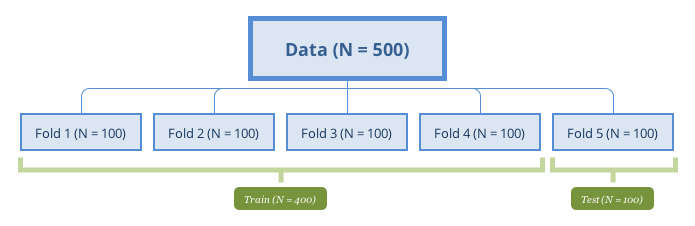
5-fold cross-validation
A special case of k-fold cross-validation is Leave One Out Cross Validation (LOOCV) where \(k=1\). When sample size is small, it is desired to use as many data to train the model. Most of the functions have default setting \(k=10\). The choice is usually 5-10 in practice, but there is no standard rule. The more folds to use, the more samples are used to fit model, and then the performance estimate is closer to the theoretical performance. Meanwhile, the variance of the performance is larger since the samples to fit model in different iterations are more similar. However, LOOCV has high computational cost since the number of interactions is the same as the sample size and each model fit uses a subset that is nearly the same size of the training set. On the other hand, when k is small (such as 2 or 3), the computation is more efficient, but the bias will increase. When the sample size is large, the impact of \(k\) becomes marginal.
Chapter 7 of (Hastie T 2008) presents a more in-depth and more detailed discussion about the bias-variance trade-off in k-fold cross-validation.
You can implement k-fold cross-validation using createFolds() in caret:
library(caret)
class <- sim.dat$segment
# creat k-folds
set.seed(1)
cv <- createFolds(class, k = 10, returnTrain = T)
str(cv)
## List of 10
## $ Fold01: int [1:900] 1 2 3 4 5 6 7 8 9 10 ...
## $ Fold02: int [1:900] 1 2 3 4 5 6 7 9 10 11 ...
## $ Fold03: int [1:900] 1 2 3 4 5 6 7 8 10 11 ...
## $ Fold04: int [1:900] 1 2 3 4 5 6 7 8 9 11 ...
## $ Fold05: int [1:900] 1 3 4 6 7 8 9 10 11 12 ...
## $ Fold06: int [1:900] 1 2 3 4 5 6 7 8 9 10 ...
## $ Fold07: int [1:900] 2 3 4 5 6 7 8 9 10 11 ...
## $ Fold08: int [1:900] 1 2 3 4 5 8 9 10 11 12 ...
## $ Fold09: int [1:900] 1 2 4 5 6 7 8 9 10 11 ...
## $ Fold10: int [1:900] 1 2 3 5 6 7 8 9 10 11 ...The above code creates ten folds (k=10) according to the customer segments (we set class to be the categorical variable segment). The function returns a list of 10 with the index of rows in training set.
7.2.2.2 Repeated Training/Test Splits
In fact, this method is nothing but repeating the training/test set division on the original data. Fit the model with the training set, and evaluate the model with the test set. Unlike k-fold cross-validation, the test set generated by this procedure may have duplicate samples. A sample usually shows up in more than one test sets. There is no standard rule for split ratio and number of repetitions. The most common choice in practice is to use 75% to 80% of the total sample for training. The remaining samples are for validation. The more sample in the training set, the less biased the model performance estimate is. Increasing the repetitions can reduce the uncertainty in the performance estimates. Of course, it is at the cost of computational time when the model is complex. The number of repetitions is also related to the sample size of the test set. If the size is small, the performance estimate is more volatile. In this case, the number of repetitions needs to be higher to deal with the uncertainty of the evaluation results.
We can use the same function (createDataPartition ()) as before. If you look back, you will see times = 1. The only thing to change is to set it to the number of repetitions.
trainIndex <- createDataPartition(sim.dat$segment,
                                  p = .8,
                                  list = FALSE,
                                  times = 5)
dplyr::glimpse(trainIndex)
## int [1:800, 1:5] 1 3 4 5 6 7 8 9 10 11 ...
## - attr(*, "dimnames")=List of 2
## ..$ : NULL
## ..$ : chr [1:5] "Resample1" "Resample2" "Resample3" "Resample4" ...Once know how to split the data, the repetition comes naturally.
7.2.2.3 Bootstrap Methods
Bootstrap is a powerful statistical tool (a little magic too). It can be used to analyze the uncertainty of parameter estimates (Efron and Tibshirani 1986) quantitatively. For example, estimate the standard deviation of linear regression coefficients. The power of this method is that the concept is so simple that it can be easily applied to any model as long as the computation allows. However, you can hardly obtain the standard deviation for some models by using the traditional statistical inference.
Since it is with replacement, a sample can be selected multiple times, and the bootstrap sample size is the same as the original data. So for every bootstrap set, there are some left-out samples, which is also called “out-of-bag samples.” The out-of-bag sample is used to evaluate the model. Efron points out that under normal circumstances (Efron 1983), bootstrap estimates the error rate of the model with more certainty. The probability of an observation \(i\) in bootstrap sample B is:
\(\begin{array}{ccc} Pr{i\in B} & = & 1-\left(1-\frac{1}{N}\right)^{N}\\ & \approx & 1-e^{-1}\\ & = & 0.632 \end{array}\)
On average, 63.2% of the observations appeared at least once in a bootstrap sample, so the estimation bias is similar to 2-fold cross-validation. As mentioned earlier, the smaller the number of folds, the larger the bias. Increasing the sample size will ease the problem. In general, bootstrap has larger bias and smaller variance than cross-validation. Efron came up the following “.632 estimator” to alleviate this bias:
\[(0.632 × original\ bootstrap\ estimate) + (0.368 × apparent\ error\ rate)\]
The apparent error rate is the error rate when the data is used twice, both to fit the model and to check its accuracy and it is apparently over-optimistic. The modified bootstrap estimate reduces the bias but can be unstable with small samples size. This estimate can also be unduly optimistic when the model severely over-fits since the apparent error rate will be close to zero. Efron and Tibshirani (Efron and Tibshirani 1997) discuss another technique, called the “632+ method,” for adjusting the bootstrap estimates.