13.2 data.table— enhanced data.frame
What is data.table? It is an R package that provides an enhanced version of data.frame. The most used object in R is data frame. Before we move on, let’s briefly review some basic characters and manipulations of data.frame:
- It is a set of rows and columns.
- Each row is of the same length and data type
- Every column is of the same length but can be of differing data types
- It has characteristics of both a matrix and a list
- It uses
[]to subset data
We will use the clothes customer data to illustrate. There are two dimensions in []. The first one indicates the row and second one indicates column. It uses a comma to separate them.
# read data
sim.dat <- readr::read_csv("http://bit.ly/2P5gTw4")
## Rows: 1000 Columns: 19
## ── Column specification ───────────────────────────────
## Delimiter: ","
## chr (3): gender, house, segment
## dbl (16): age, income, store_exp, online_exp, store...
##
## ℹ Use `spec()` to retrieve the full column specification for this data.
## ℹ Specify the column types or set `show_col_types = FALSE` to quiet this message.# subset the first two rows
sim.dat[1:2, ]
# subset the first two rows and column 3 and 5
sim.dat[1:2, c(3, 5)]
# get all rows with age>70
sim.dat[sim.dat$age > 70, ]
# get rows with age> 60 and gender is Male select column 3 and 4
sim.dat[sim.dat$age > 68 & sim.dat$gender == "Male", 3:4]Remember that there are usually different ways to conduct the same manipulation. For example, the following code presents three ways to calculate an average number of online transactions for male and female:
tapply(sim.dat$online_trans, sim.dat$gender, mean)

aggregate(online_trans ~ gender, data = sim.dat, mean)

sim.dat %>%
  group_by(gender) %>%
  summarise(Avg_online_trans = mean(online_trans))
There is no gold standard to choose a specific function to manipulate data. The goal is to solve the real problem, not the tool itself. So just use whatever tool that is convenient for you.
The way to use [] is straightforward. But the manipulations are limited. If you need more complicated data reshaping or aggregation, there are other packages to use such as dplyr, reshape2, tidyr etc. But the usage of those packages are not as straightforward as []. You often need to change functions. Keeping related operations together, such as subset, group, update, join etc, will allow for:
- concise, consistent and readable syntax irrespective of the set of operations you would like to perform to achieve your end goal
- performing data manipulation fluidly without the cognitive burden of having to change among different functions
- by knowing precisely the data required for each operation, you can automatically optimize operations effectively
data.table is the package for that. If you are not familiar with other data manipulating packages and are interested in reducing programming time tremendously, then this package is for you.
Other than extending the function of [], data.table has the following advantages:
- Offers fast import, subset, grouping, update, and joins for large data files
- It is easy to turn data frame to data table
- Can behave just like a data frame
You need to install and load the package:
Use data.table() to convert the existing data frame sim.dat to data table:
dt <- data.table(sim.dat)
class(dt)
## [1] "data.table" "data.frame"Calculate mean for counts of online transactions:
dt[, mean(online_trans)]## [1] 13.55You can’t do the same thing using data frame:
sim.dat[,mean(online_trans)]Error in mean(online_trans) : object 'online_trans' not foundIf you want to calculate mean by group as before, set “by =” argument:
dt[ , mean(online_trans), by = gender]## gender V1
## 1: Female 15.38
## 2: Male 11.26You can group by more than one variables. For example, group by “gender” and “house”:
dt[ , mean(online_trans), by = .(gender, house)]## gender house V1
## 1: Female Yes 11.312
## 2: Male Yes 8.772
## 3: Female No 19.146
## 4: Male No 16.486Assign column names for aggregated variables:
dt[ , .(avg = mean(online_trans)), by = .(gender, house)]## gender house avg
## 1: Female Yes 11.312
## 2: Male Yes 8.772
## 3: Female No 19.146
## 4: Male No 16.486data.table can accomplish all operations that aggregate() and tapply()can do for data frame.
- General setting of
data.table
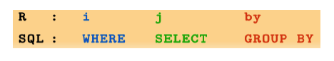
Different from data frame, there are three arguments for data table:

It is analogous to SQL. You don’t have to know SQL to learn data table. But experience with SQL will help you understand data table. In SQL, you select column j (use command SELECT) for row i (using command WHERE). GROUP BY in SQL will assign the variable to group the observations.
Let’s review our previous code:
dt[ , mean(online_trans), by = gender]The code above is equal to the following SQL:
SELECT
   gender,
   avg(online_trans)
FROM
   sim.dat
GROUP BY
   gender
R code:
dt[ , .(avg = mean(online_trans)), by = .(gender, house)]is equal to SQL:
SELECT
   gender,
   house,
   avg(online_trans) AS avg
FROM
   sim.dat
GROUP BY
   gender,
   house
R code:
dt[ age < 40, .(avg = mean(online_trans)), by = .(gender, house)]is equal to SQL:
SELECT
   gender,
   house,
   avg(online_trans) AS avg
FROM
   sim.dat
WHERE
   age < 40
GROUP BY
   gender,
   house
You can see the analogy between data.table and SQL. Now let’s focus on operations in data table.
- select row
# select rows with age<20 and income > 80000
dt[age < 20 & income > 80000]
## age gender income house store_exp online_exp
## 1: 19 Female 83535 No 227.7 1491
## 2: 18 Female 89416 Yes 209.5 1926
## 3: 19 Female 92813 No 186.7 1042
## store_trans online_trans Q1 Q2 Q3 Q4 Q5 Q6 Q7 Q8 Q9
## 1: 1 22 2 1 1 2 4 1 4 2 4
## 2: 3 28 2 1 1 1 4 1 4 2 4
## 3: 2 18 3 1 1 2 4 1 4 3 4
## Q10 segment
## 1: 1 Style
## 2: 1 Style
## 3: 1 Style# select the first two rows
dt[1:2]## age gender income house store_exp online_exp
## 1: 57 Female 120963 Yes 529.1 303.5
## 2: 63 Female 122008 Yes 478.0 109.5
## store_trans online_trans Q1 Q2 Q3 Q4 Q5 Q6 Q7 Q8 Q9
## 1: 2 2 4 2 1 2 1 4 1 4 2
## 2: 4 2 4 1 1 2 1 4 1 4 1
## Q10 segment
## 1: 4 Price
## 2: 4 Price- select column
Selecting columns in data.table don’t need $:
# select column “age” but return it as a vector
# the argument for row is empty so the result
# will return all observations
ans <- dt[, age]
head(ans)
## [1] 57 63 59 60 51 59To return data.table object, put column names in list():
# Select age and online_exp columns
# and return as a data.table instead
ans <- dt[, list(age, online_exp)]
head(ans)
Or you can also put column names in .():
ans <- dt[, .(age, online_exp)]To select all columns from “age” to “income”:
ans <- dt[, age:income, with = FALSE]
head(ans,2)
## age gender income
## 1: 57 Female 120963
## 2: 63 Female 122008Delete columns using - or !:
# delete columns from  age to online_exp
ans <- dt[, -(age:online_exp), with = FALSE]
ans <- dt[, !(age:online_exp), with = FALSE]- tabulation
In data table. .N means to count。
# row count
dt[, .N]
## [1] 1000If you assign the group variable, then it will count by groups:
# counts by gender
dt[, .N, by= gender]
## gender N
## 1: Female 554
## 2: Male 446# for those younger than 30, count by gender
dt[age < 30, .(count=.N), by= gender] ## gender count
## 1: Female 292
## 2: Male 86Order table:
# get records with the highest 5 online expense:
head(dt[order(-online_exp)],5)
age gender income house store_exp online_exp store_trans ...
1: 40 Female 217599.7 No 7023.684 9479.442 10
2: 41 Female NA Yes 3786.740 8638.239 14
3: 36 Male 228550.1 Yes 3279.621 8220.555 8
4: 31 Female 159508.1 Yes 5177.081 8005.932 11
5: 43 Female 190407.4 Yes 4694.922 7875.562 6
...Since data table keep some characters of data frame, they share some operations:
dt[order(-online_exp)][1:5]You can also order the table by more than one variable. The following code will order the table by gender, then order within gender by online_exp:
dt[order(gender, -online_exp)][1:5]- Use
fread()to import dat
Other than read.csv in base R, we have introduced ‘read_csv’ in ‘readr’. read_csv is much faster and will provide progress bar which makes user feel much better (at least make me feel better). fread() in data.table further increase the efficiency of reading data. The following are three examples of reading the same data file topic.csv. The file includes text data scraped from an agriculture forum with 209670 rows and 6 columns:
system.time(topic <- read.csv("http://bit.ly/2zam5ny")) user system elapsed
3.561 0.051 4.888 system.time(topic <- readr::read_csv("http://bit.ly/2zam5ny")) user system elapsed
0.409 0.032 2.233 system.time(topic <- data.table::fread("http://bit.ly/2zam5ny")) user system elapsed
0.276 0.096 1.117 It is clear that read_csv() is much faster than read.csv(). fread() is a little faster than read_csv(). As the size increasing, the difference will become for significant. Note that fread() will read file as data.table by default.