4.3 Introduction of Cloud Environment
Even though Spark provides a solution for big data analytics, the maintenance of the computing cluster and Spark system requires a dedicated team. Historically for each organization the IT departments own the hardware and the regular maintenance. It usually takes months for a new environment to be built and the cost is high. Luckily, the time to deployment and cost are dramatically down due to the cloud computation trend. Now we can create a Spark computing cluster in the cloud in a few minutes with the desired configuration and the user only pay when the cluster is up. Cloud computing environments enable smaller organizations to adopt big data analytics.
There are many cloud computing environments such as Amazon’s AWS, Google cloud and Microsoft Azure which provide a complete list of functions for heavy-duty enterprise applications. For example, Netflix runs its business entirely on AWS without owning any data centers. For beginners, however, Databricks provides an easy to use cloud system for learning purposes. Databricks is a company founded by the creators of Apache Spark and it provides a user-friendly web-based notebook environment that can create a Spark cluster on the fly to run R/Python/Scala/SQL scripts. We will use Databricks’ free community edition to run demos in this book. Please note, to help readers to get familiar with the Databricks cloud system, the content of this section is partially adopted from the following web pages:
4.3.1 Open Account and Create a Cluster
Anyone can apply for a free Databrick account through https://databricks.com/try-databricks and please make sure to choose the “COMMUNITY EDITION” which does not require payment information and will always be free. Once the community edition account is open and activated. Users can create a cluster computation environment with Spark. The computing cluster associated with community edition account is relatively small, but it is good enough for running all the examples in this book. The main user interface to the computing environment is notebook: a collection of cells that contains formatted text or codes. When a new notebook is created, user will need to choose the default programming language type (i.e. Python, R, Scala, or SQL) and every cells in the notebook will assume the default programming language. However, user can easily override the default selection of programming language by adding %sql, %python, %r or %scala at the first line of each cell to indicate the programming language in that cell. Allowing running different cells with different programming language in the same notebook enable user to have the flexibility to choose the best tools for each task. User can also define a cell to be markdown cell by adding %md at the first line of the cell. A markdown cell does not performance computation and it is just a cell to show formatted text. Well separated cells with computation, graph and formatted text enable user to create easy to maintain reproducible reports. The link to a video showing how to open Databricks account, how to create a cluster, and how to create notebooks is included in the book’s website.
4.3.2 R Notebook
For this book, we will use R notebook for examples and demos and the corresponding Python notebook will be available online too. For an R notebook, it contains multiple cells, and, by default, the content within each cell are R scripts. Usually, each cell is a well-managed segment of a few lines of codes that accomplish a specific task. For example, Figure 4.2 shows the default cell for an R notebook. We can type in R scripts and comments same as we are using R console. By default, only the result from the last line will be shown following the cell. However, you can use print() function to output results for any lines. If we move the mouse to the middle of the lower edge of the cell below the results, a “+” symbol will show up and click on the symbol will insert a new cell below. When we click any area within a cell, it will make it editable and you will see a few icons on the top right corn of the cell where we can run the cell, as well as add a cell below or above, copy the cell, cut the cell etc. One quick way to run the cell is Shift+Enter when the cell is chosen. User will become familiar with the notebook environment quickly.
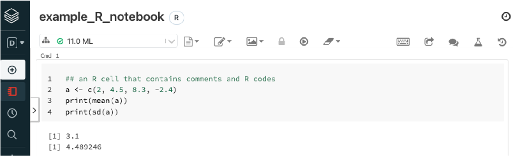
FIGURE 4.2: Example of R Notebook
4.3.3 Markdown Cells
For an R notebook, every cell by default will contain R scripts. But if we put %md, %sql or %python at the first line of a cell, that cell becomes Markdown cell, SQL script cell, and Python script cell accordingly. For example, Figure 4.3 shows a markdown cell with scripts and the actual appearance when exits editing mode. Markdown cell provides a straightforward way to descript what each cell is doing as well as what the entire notebook is about. It is a better way than a simple comment within the code.
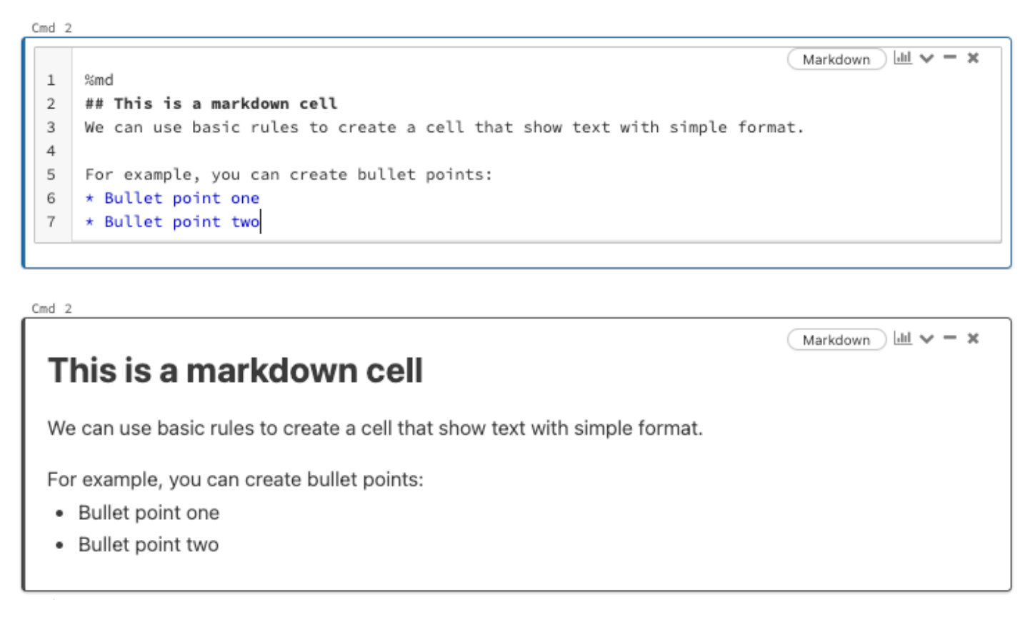
FIGURE 4.3: Example of Markdown Cell